Fix ADDRESS and INDIRECT mix-ups in Google Sheets (A1, R1C1, absolute mode)

ADDRESS(row, column, [absolute_relative_mode], [use_a1_notation], [sheet]) returns text, not a cell. Mode 1 is $A$1. Mode 4 is A1. The fourth argument is not another mode number: TRUE means A1 notation, FALSE means R1C1. INDIRECT reads that text. Its default is A1. An R1C1 string fed to that default is #REF!. A mode of 0 never gets that far: ADDRESS itself is #NUM!.

This page is notation and the absolute mode. It is not INDIRECT #REF! as a general bad string ("not an address"). It is not INDIRECT sheet name (spaces and apostrophes in the tab). It is not OFFSET height / width. Keep the Google Sheets UI in English.

Recreate it on a blank sheet

1. Open a blank spreadsheet. In A1 type origin. In C2 type target. You want text that points at C2, then a formula that reads C2 through that text.

Absolute A1, the control. In E1 type a1. In E2 enter =ADDRESS(2,3,1,TRUE). The cell shows $C$2. Row 2, column 3, mode 1 (both locks), A1 notation. In E3 enter =INDIRECT(E2). The cell shows target. That pair is the control.

Relative mode is not “R1C1”. In E5 type mode4. In E6 enter =ADDRESS(2,3,4,TRUE). The cell shows C2 with no dollar signs. Mode 4 is still A1 notation. It is relative text. INDIRECT of C2 still returns target, because the text is a legal A1 address. People pass 4 expecting R1C1 and then lock the wrong thing when they copy a formula that embeds that text. Leave E6 as C2 so you can see the missing dollars. It is not an error triangle.

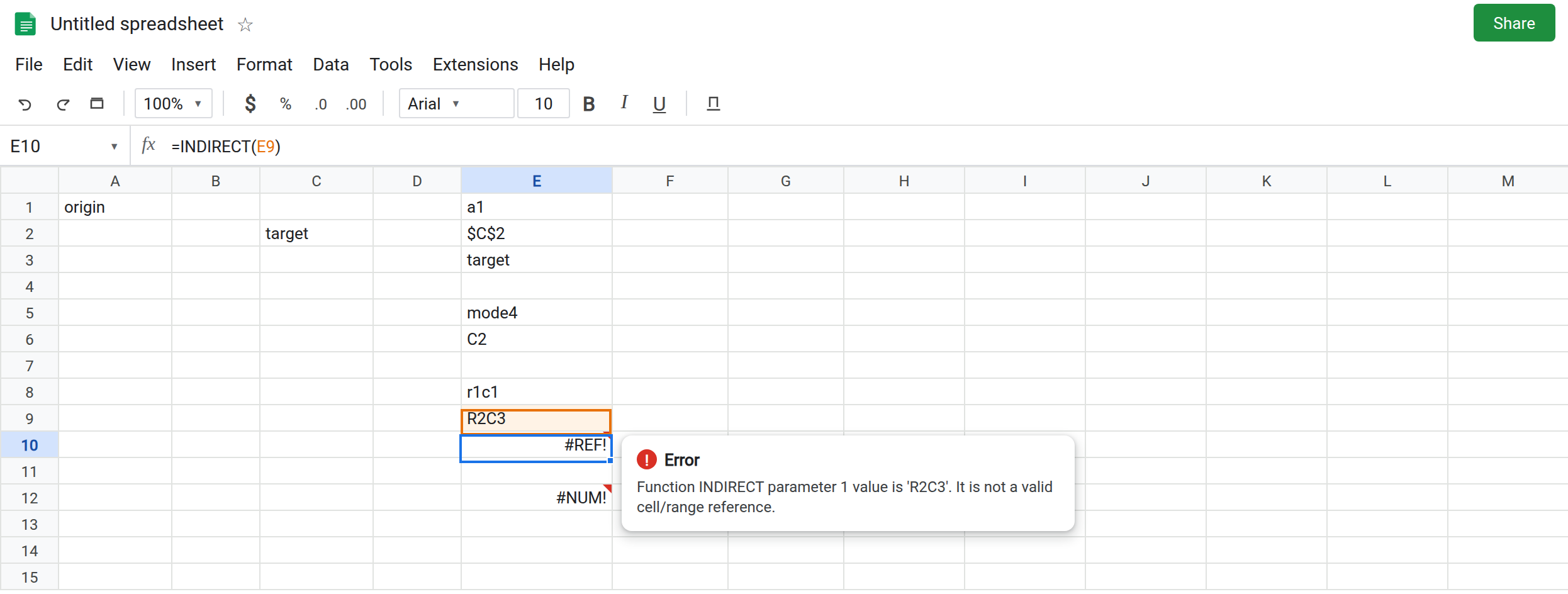
FALSE is R1C1. In E8 type r1c1. In E9 enter =ADDRESS(2,3,1,FALSE). The cell shows R2C3. Fourth argument FALSE, not a mode. In E10 enter =INDIRECT(E9). The cell shows #REF!. INDIRECT defaults to A1 notation. R2C3 is not an A1 address. Leave E10 broken.

Mode 0. In E12 enter =ADDRESS(2,3,FALSE). FALSE coerces to 0. The third argument must be 1, 2, 3, or 4. The cell shows #NUM!. The tooltip says parameter 3 should be between 1 and 4. People pass FALSE to mean “not absolute” and hit this before any INDIRECT. Leave E12 broken.

Relative R1C1 text. In G1 type rel. In G2 enter =ADDRESS(2,3,4,FALSE). The cell shows an R1C1 relative form with brackets, such as R[2]C[3], not R2C3. Those brackets are offsets, not “row 2, column 3” as a fixed cell. INDIRECT of that string is a different cell than C2, or #REF!, depending on where the formula sits. Leave G2 as the bracket text. Do not treat it as a synonym of E9.

Sheet text is still text. In G4 enter =ADDRESS(2,3,1,TRUE,"Dock List"). The cell shows 'Dock List'!$C$2. Quoting the tab is ADDRESS’s job when you pass the sheet name. A space in a name you concatenate yourself is INDIRECT sheet name.

Leave E10 and E12 broken. Leave E3 as target.

What is actually wrong

• ADDRESS does not read C2. It writes a label. INDIRECT is what reads. A pretty label in the wrong notation is E10.
• Argument 3 is the lock mode. 1 both absolute, 2 row absolute and column relative (C$2), 3 row relative and column absolute ($C2), 4 both relative (C2). Argument 4 is the notation flag. Swapping those ideas is this page.
• FALSE in argument 3 is mode 0, which is #NUM! (E12). FALSE in argument 4 is R1C1 (E9).
• INDIRECT(ref, is_A1) uses A1 when is_A1 is omitted or TRUE. R1C1 text needs FALSE there. The string can be perfect and the second argument still wrong.
• Relative R1C1 with brackets is not absolute R2C3. Copying G2 into INDIRECT does not mean “always C2”.
• Row or column 0 on ADDRESS is also #NUM!. Rows start at 1. That is the same family as E12, not a notation bug.

This is not a deleted cell. See after you delete. E10’s formula still says INDIRECT(E9).

This is not OFFSET walking off the sheet. See OFFSET off sheet. ADDRESS never walks. It only returns text.

Fix

Leave E10 and E12 broken.

A1 text, A1 indirect. Keep E2 and E3: =ADDRESS(2,3,1,TRUE) and =INDIRECT(E2). If you need a relative A1 label on purpose, E6 is already C2, and =INDIRECT(E6) returns target.

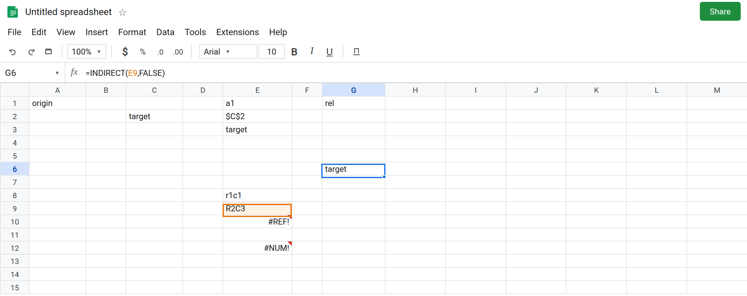
R1C1 text needs the flag on INDIRECT. In G6 enter =INDIRECT(E9,FALSE). The second argument is FALSE. The cell shows target. E9 stays R2C3. You did not convert E9 back to $C$2. You told INDIRECT how to read it.

Pass a real mode. Absolute A1 is mode 1, not FALSE. Relative A1 is mode 4 with the fourth argument TRUE or omitted. Do not pass FALSE in the mode slot.

Do not wrap E10 in IFERROR. You would hide an R1C1 string that is one argument away from working. See IFERROR vs IFNA.

If ADDRESS is #NUM!, the mode is not 1–4 or the row/column is below 1. If ADDRESS looks like R2C3 and INDIRECT is #REF!, pass FALSE as INDIRECT’s second argument, or build A1 text with mode 1 and TRUE.