IFERROR hides the real error in Google Sheets: how to see the cause

IFERROR(value, [fallback]) replaces every error with the fallback. Omit the fallback and the replacement is blank. A column of blanks or zeros can be a missing sku, a column index past the range, a divide by zero, or a mistyped function, and the grid will not say which. The way out is to calculate the inside formula in a scratch cell, read the token and the tooltip, fix that error, and only then decide whether a wrapper still belongs. IFNA is narrower. It is not a diagnostic. It is a different wrapper.

This page is how to open a formula that already hides its cause. The side-by-side of the two wrappers is IFERROR vs IFNA. Keep the Google Sheets UI in English.

Recreate it on a blank sheet

1. Open a blank spreadsheet. In A1 type sku, B1 name, C1 qty. A2 101, B2 Widget, C2 0. In E1 type key. E2 999.

Three different failures, one wrapper. In G1 type raw_na. In G2 enter =VLOOKUP(E2,A2:B2,2,FALSE). G2 is #N/A. The key 999 is absent. In G4 enter =VLOOKUP(A2,A2:B2,3,FALSE). G4 is #REF!. The key 101 exists. Index 3 does not. In G6 enter =1/C2. G6 is #DIV/0!. Leave all three.

The wrapper they get pasted into. In I1 type hidden. In I2 enter =IFERROR(VLOOKUP(E2,A2:B2,2,FALSE),0). In I4 enter =IFERROR(VLOOKUP(A2,A2:B2,3,FALSE),0). In I6 enter =IFERROR(1/C2,0). I2, I4, and I6 all show 0. A sum of that column is 0. Nothing in the column says miss, bad index, or zero qty. Leave I2:I6 as that false calm.

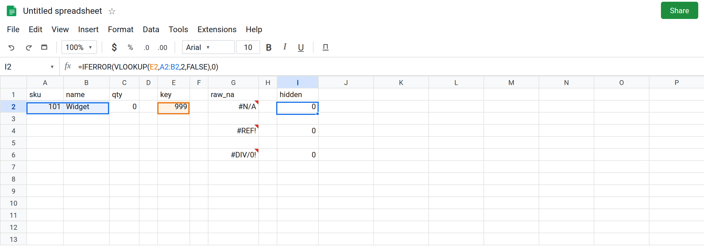
A blank fallback hides even the zero. In I8 enter =IFERROR(1/C2). No second argument. I8 is blank, not 0, not #DIV/0!. A blank is easy to read as “no row.” C2 is a zero qty on a row that exists. Leave I8 blank.

Nested wrappers. In I10 enter =IFERROR(VLOOKUP(E2,A2:B2,2,FALSE),IFERROR(1/C2,0)). I10 shows 0. The lookup missed, so the second IFERROR ran, divided by zero, and also failed. You cannot tell which branch produced the 0. Leave I10 as 0.

IFNA does not open the diagnosis by itself, but it stops the lie. In K2 enter =IFNA(VLOOKUP(A2,A2:B2,3,FALSE),0). K2 stays #REF!. The bad index is still visible. IFNA would turn G2 into 0 and would leave G6 as #DIV/0!. That comparison is IFERROR vs IFNA. Leave K2 as #REF!.

Leave I2, I4, and I6 as 0. Leave G2, G4, and G6 as the three tokens.

What is actually wrong

• The fallback is one value for many causes. 0 means “someone chose 0,” not “Sheets found a zero.” I2 is a miss. I4 is a range error. I6 is arithmetic. The column cannot be charted or summed as if those were measurements.
• Blank is a fallback too. I8. COUNTA skips it. COUNTBLANK counts it. A report of “empty imports” may be counting errors you wrapped.
• Nested IFERROR runs the next attempt only when the first errors, then wraps that attempt as well. I10 collapses two failures. Split them into two scratch cells before you trust the 0.
• The wrapper is not the bug you fix first. G4’s index is VLOOKUP bad index. G6 is divide by zero. G2, once you accept that 999 is absent, may keep a wrapper — and that wrapper should be IFNA, not IFERROR, so a future bad index still shows.
• IFERROR around IMPORTRANGE hides Allow access. See IMPORTRANGE access. Peel that one too. Click Allow access. Do not replace the banner with 0.
• A #NAME? from VLOKUP becomes 0 under IFERROR. See unknown function. The scratch cell shows the unknown name. The wrapped cell does not.

Fix

Leave I2:I6 wrapped so the contrast stays. Do the reading on the G column.

Copy the inside into a scratch cell. G2, G4, and G6 are already that copy. For a formula you did not build twice: select I2, copy the text inside the parentheses (the VLOOKUP, not IFERROR and not ,0) into M2. M2 shows #N/A and the tooltip names 999. That is the cause for this row.

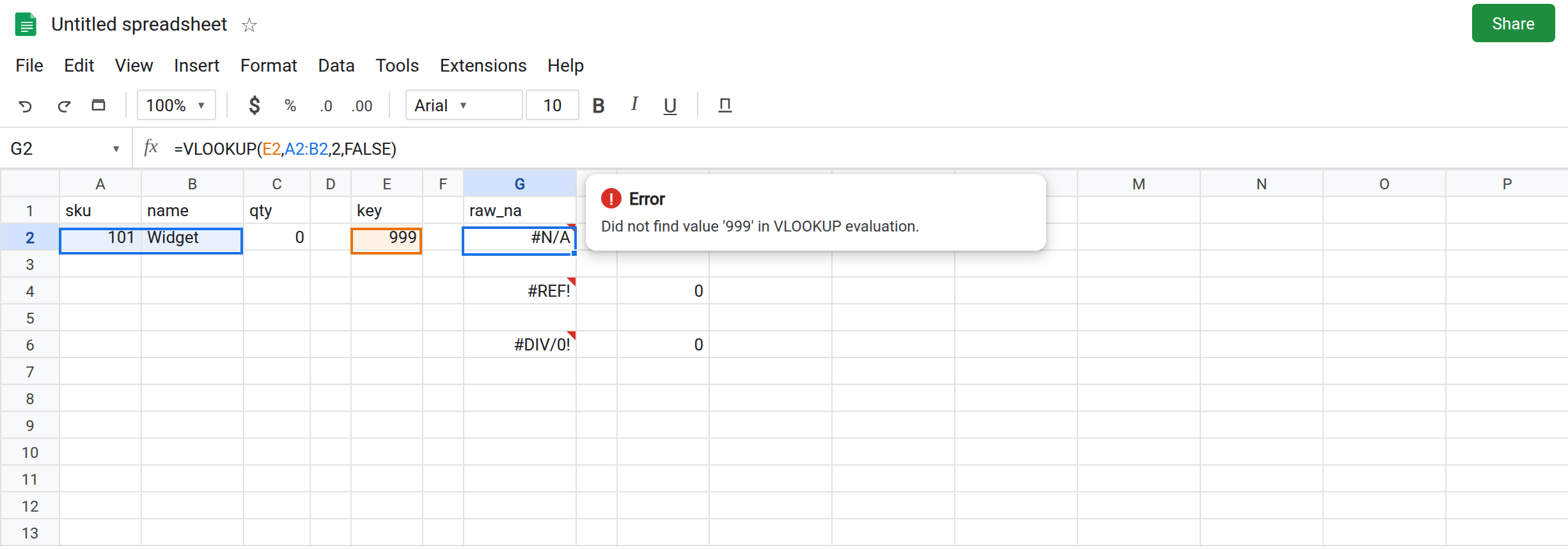
Fix the cause, then choose a wrapper only if a miss is allowed. Index 2 for the name: =VLOOKUP(A2,A2:B2,2,FALSE) is Widget. Qty in C2 must be non-zero before you divide; guard with =IF(C2=0,"",1/C2) rather than IFERROR. For a key that is allowed to be absent, =IFNA(VLOOKUP(E2,A2:B2,2,FALSE),0) turns only #N/A into 0. Point it at G4’s formula and the #REF! remains. That is the check that the wrapper is narrow enough.

One wrapper, last. Do not nest I10. Two scratch cells, two fixes. If both are deliberate fallbacks, they still deserve two columns so a reader can see which one fired.

If a column is uniformly 0 or blank and the formula bar starts with IFERROR, peel one cell. Match the raw token to its page. Put IFERROR back only when every error in that cell should look the same, which is rare for a lookup. A lookup that is allowed to miss uses IFNA or XLOOKUP’s missing-value argument. See XLOOKUP no match.