CHOOSECOLS with a negative index follows the right edge, so an added column changes the pick

CHOOSECOLS counts columns inside the range in the formula. 1 is the first column of that range. -1 is the last. It is not “the price column,” and it is not the last column of the sheet. Append a notes column and extend the range, and -1 returns notes. The prices are still there. The index means a different field, and there is no error.

Index 0, and a negative whose absolute value is larger than the width, are CHOOSEROWS negative. Sheet-column numbers versus relative indexes are CHOOSEROWS / CHOOSECOLS. Keep the Google Sheets UI in English. Sheet Error is an independent formula-error library, not a Google product.

Recreate it on a blank sheet

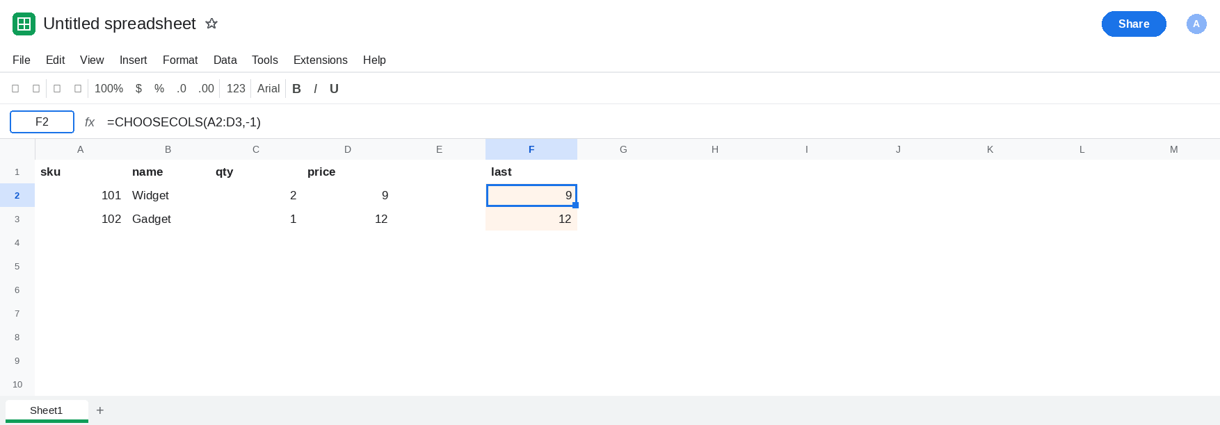
1. Open a blank spreadsheet. In A1 type sku, B1 name, C1 qty, D1 price. A2 101, B2 Widget, C2 2, D2 9. A3 102, B3 Gadget, C3 1, D3 12. Four columns. Price is last. The range is A2:D3.

Negative one is price. Leave F2:F3 empty. In F1 type last. In F2 enter =CHOOSECOLS(A2:D3,-1). The spill is 9 and 12. In F5 enter =CHOOSECOLS(A2:D3,4). F5:F6 is also 9 and 12. On this range, -1 and 4 are the same column. F2 is the control.

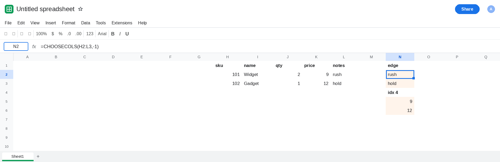
Notes appended on the right. In H1 type sku, I1 name, J1 qty, K1 price, L1 notes. H2 101, I2 Widget, J2 2, K2 9, L2 rush. H3 102, I3 Gadget, J3 1, K3 12, L3 hold. Five columns. Price is fourth. Notes are last. In N1 type edge. In N2 enter =CHOOSECOLS(H2:L3,-1). The spill is rush and hold. Not 9 and 12. There is no error triangle. In N5 enter =CHOOSECOLS(H2:L3,4). N5:N6 is 9 and 12. Index 4 is still price, because notes were added after it. -1 moved. -2 is the price on this range: in N8 enter =CHOOSECOLS(H2:L3,-2). N8:N9 is 9 and 12. Leave N2 as the notes.

A column inserted in front of price moves index 4. In H6 type sku, I6 name, J6 qty, K6 notes, L6 price. H7 101, I7 Widget, J7 2, K7 rush, L7 9. H8 102, I8 Gadget, J8 1, K8 hold, L8 12. Price is last again, so -1 is price. Index 4 is notes. In N11 enter =CHOOSECOLS(H7:L8,4). The spill is rush and hold. In N14 enter =CHOOSECOLS(H7:L8,-1). The spill is 9 and 12. The insert in the middle broke the positive index and left the negative one on the price. The append in H1:L3 did the opposite. Leave both spills.

You do not have to use Insert → Column to see this. Those two blocks are the shapes Sheets leaves behind: a range that grew on the right, and a range that grew in the middle. A live A2:D3 expands when you insert inside it. -1 follows whatever the right edge is after that expansion.

What is actually wrong

• Negative indexes count from the right of the range argument. -1 on A2:D3 is D. -1 on H2:L3 is L. CHOOSECOLS(B2:D3,-1) is still D, the last of those three columns, not a column out past Z.
• Appending a column changes -1 and does not change an index that still points at the same field. N2 is notes. N5 is still the price. People switch to -1 so inserts on the left will not bother them. An extra column on the right is exactly what -1 cannot ignore.
• Inserting in front of the field does the other damage. N11 is index 4 landing on notes. -1 on that block is still the price, because price is still last.
• -5 on a four-column range is out of range. The whole call errors. That tooltip is CHOOSEROWS negative. N2 is in range. It is the wrong field.
• SUM of N2 is #VALUE! once the spill is text. The formula did not fail. The column did.

Fix

Leave N2 as the notes.

Find the header, then choose that position. In P1 type by name. In P2 enter =CHOOSECOLS(H2:L3,MATCH("price",H1:L1,0)). MATCH returns 4. CHOOSECOLS returns 9 and 12. In P5 enter =CHOOSECOLS(H7:L8,MATCH("price",H6:L6,0)). The header price is now in column L, position 5. P5:P6 is 9 and 12. The same pattern works on both layouts. A notes column does not become the price unless you rename the header.

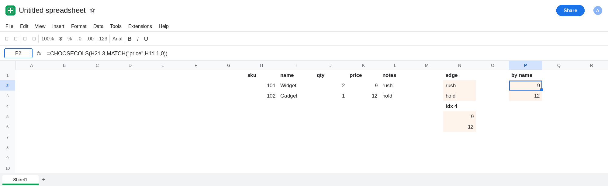
Use -1 only when last really means the field you want. Keep F2 while price is the right edge of A2:D3 and you will not extend that range. The moment notes share the range, -1 is notes. -2 is a guess about how the columns will grow. The header match is the one that survives both inserts.

Do not wrap N2 in IFERROR. Notes are a successful result. See IFERROR vs IFNA.

If -1 returns a label you added on the right, the index is following the new edge. Match the header. If a positive index returns the inserted column, the insert landed to the left of the field and the number is stale. If the tooltip says the index is outside 1 through the width, the negative went past the first column, and you are on the out-of-range page.