Formula parse error in Google Sheets (comma vs semicolon, locale)

You paste a VLOOKUP from a US tutorial and the cell shows #ERROR!. The tooltip says Formula parse error. The function name is fine. The commas are not. Any function with more than one argument hits the same wall on this locale: IF, MATCH, SUMIF. The spreadsheet locale owns the argument separator, not the tutorial you copied.

Recreate it on a blank sheet

1. Open a new blank spreadsheet. File > Settings > Locale → Germany (or Deutsch / Germany). Reload the spreadsheet so the locale actually applies.
2. In A2 type 101. B2 Widget. D2 101. In A3 type 1,2 so the decimal comma is visible on the sheet. Leave A3 out of the formula.
3. In E2 paste exactly =VLOOKUP(D2,A2:B2,2,FALSE) with commas. The cell shows #ERROR!. The tooltip is Formula parse error.

E2 selected. Formula bar shows =VLOOKUP(D2,A2,2,FALSE). E2 is #ERROR! with tooltip Formula parse error.

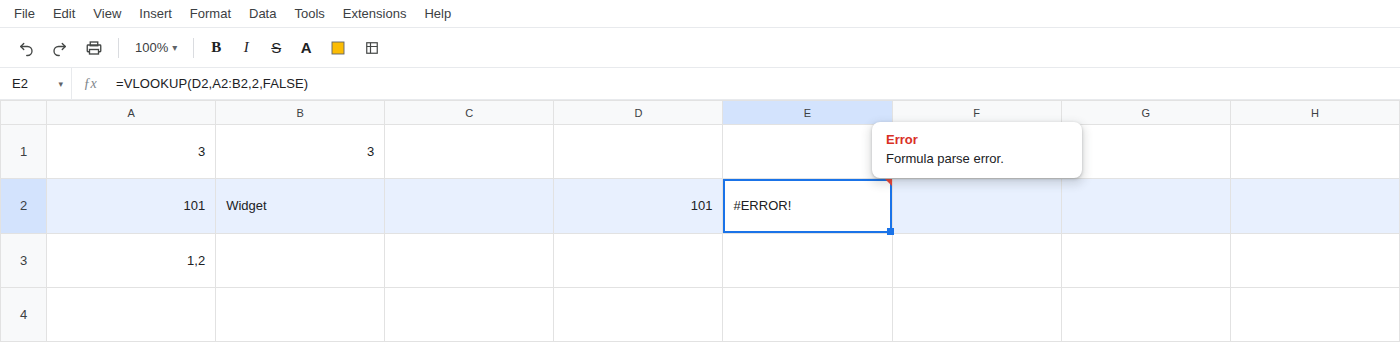
Leave E2 as the broken formula.

Second recreate — IF with the same commas. In G1 type if. In G2 enter =IF(D2=101,B2,"none") with commas. The cell shows #ERROR!. Same tooltip. IF is spelled correctly. The arguments are the ones you meant. Germany uses a comma as the decimal mark, so a comma cannot also separate arguments. Four-argument VLOOKUP is the parse error you actually get from a US paste. Two-argument IF proves it is not a VLOOKUP bug.

=SUM(1,2) is a bad demo. On a German locale that can display as 1,2 (a decimal) and never error. Do not use SUM of two literals to test this.

What is actually wrong

The argument separator follows this spreadsheet’s locale, not the locale of whoever wrote the tutorial you copied, and not your Google account language. US and UK sheets use commas between arguments. Locales that use a comma as the decimal mark (Germany, France, Brazil, and many others) use semicolons between arguments.

Changing locale does not rewrite formulas already on the sheet. A comma VLOOKUP that worked last week is still commas after you switch this file to Germany. It becomes #ERROR! on reload. The function name did not break.

This page is function arguments. Separators inside { } are different: a US comma between columns becomes a backslash on this locale, not a semicolon. {A2;B2} stacks rows. {A2\B2} is two columns. See array literal locale. Do not apply the semicolon fix inside an array literal and assume you kept the same shape.

This is not #NAME?. #NAME? is an unknown function (VLOKUP). See unknown function. VLOOKUP and IF are spelled correctly here. The tooltip is Formula parse error, not Unknown function.

This is not QUERY Unable to parse query string. That error is #VALUE! inside the query language (quotes, dates, Col vs A). See QUERY parse string. E2 never got as far as running VLOOKUP.

This is not #N/A. Nothing was looked up. See what #N/A means. This is not a spill #REF!. See SORT / UNIQUE spill.

Fix

Leave E2 and G2 as the broken formulas so the parse error stays on the sheet.

In F2 enter =VLOOKUP(D2;A2:B2;2;FALSE) with semicolons. The cell shows Widget.

F2 selected. Formula bar shows =VLOOKUP(D2;A2;2;FALSE). F2 is Widget. E2 is still #ERROR!.

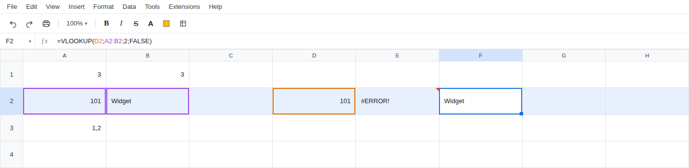
In H2 enter =IF(D2=101;B2;"none") with semicolons. The cell shows Widget.

Do not change your Google account language. Do not wrap E2 in IFERROR. The only settings change is this spreadsheet: File > Settings > Locale, then reload. For a sheet you will keep, type the separators this locale expects. If you would rather keep US separators, set the locale back to United States and reload, then leave the commas.