QUERY format datetime patterns use MM for month and mm for minutes

QUERY can end with format. For a datetime column the pattern is not the spreadsheet’s date menu, and it is not the letter rules inside TEXT. In this pattern MM is the month and mm is the minutes. HH is the hour from 00 to 23. hh is the hour from 01 to 12. The string people paste from a TEXT habit, format A 'yyyy-mm-dd hh:mm', runs. It does not mean year, month, day, and 24-hour time. A timestamp of 6 May 2024 at 15:04 can come back with 04 in the month slot and 03 in the hour slot, because those letters asked for minutes and a 12-hour clock.

The formatted cell is text, the same outcome as a numeric format on QUERY format. A date literal inside where is QUERY date literal. Keep the Google Sheets UI in English. Sheet Error is an independent formula-error library, not a Google product. Locale United States.

Recreate it on a blank sheet

1. Open a blank spreadsheet. In A1 type when, B1 sku. In A2 enter =DATE(2024,5,6)+TIME(15,4,0). B2 101. In A3 enter =DATE(2024,5,6)+TIME(9,5,0). B3 102. Format A2:A3 as Format → Number → Date time if they show serials. The formula bar still shows a date and a time, not text. ISNUMBER(A2) is TRUE. 6 May 2024, 15:04 and 09:05.

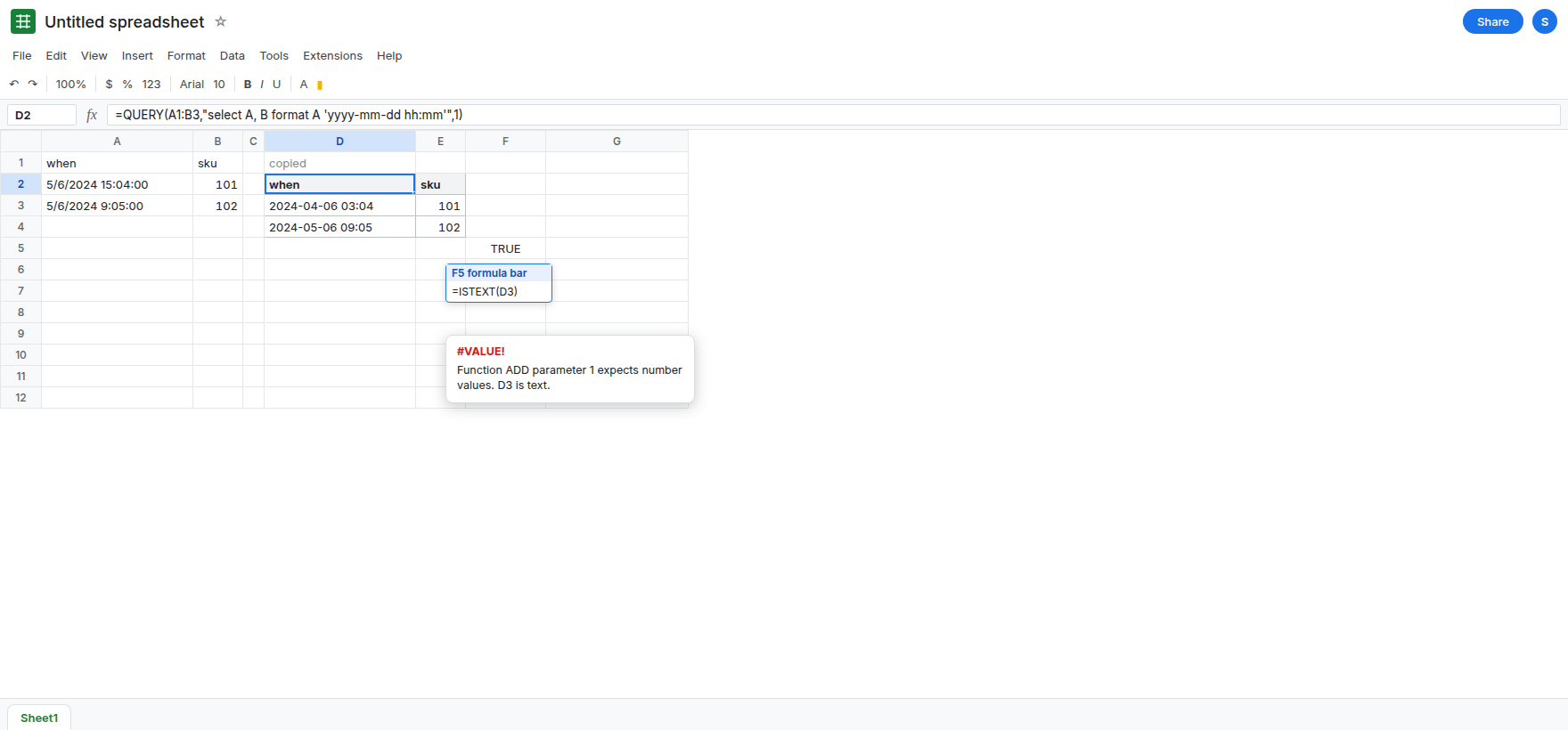
The pattern copied from TEXT. In D1 type copied. In D2 enter =QUERY(A1:B3,"select A, B format A 'yyyy-mm-dd hh:mm'",1). The spill has a header and two rows. Look at the formatted timestamp for sku 101. The month slot is not 05. It follows the minutes (04 at 15:04). The hour is on a 12-hour clock (03, not 15). Sku 102 at 09:05 shows minutes 05 in the month slot. There is no #VALUE!. The clause applied. It applied the letters you wrote. In F5 enter =ISTEXT on the formatted timestamp cell. It is TRUE. In F6 enter = that cell +1. F6 is #VALUE!. The stamp is no longer a serial. Leave D2 as this spill and leave F6 broken.

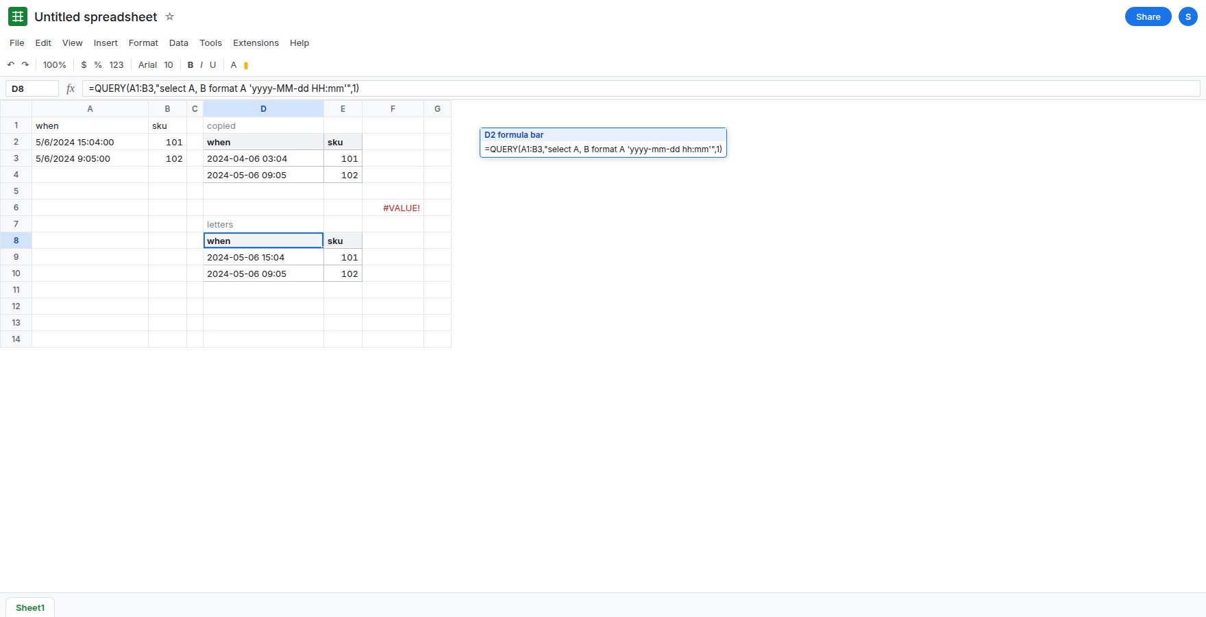
Month and 24-hour letters. In D7 type letters. In D8 enter =QUERY(A1:B3,"select A, B format A 'yyyy-MM-dd HH:mm'",1). The 101 row reads 2024-05-06 15:04. The 102 row reads 2024-05-06 09:05. MM is the month. HH is 00–23. That block is the control. It is still text. +1 on it is #VALUE! for the same reason as F6.

Text that only looks like a timestamp. In A5 type '2024-05-06 15:04 with a leading apostrophe. B5 103. ISNUMBER(A5) is FALSE. In D11 enter =QUERY(A5:B5,"select A format A 'yyyy-MM-dd HH:mm'",0). The third argument is 0 because this range has no header. The spill shows the original text. The pattern has no datetime to format. This is the case that looks ignored. Leave D11 as that unchanged text. Real datetimes are A2:A3. See dates stored as text.

The sheet locale does not rewrite the pattern. File → Settings → Locale changes how A2 is painted in the grid. It does not turn mm into a month inside the quotes, and it does not turn D8’s text back into a serial. See ambiguous date display for the grid, and QUERY format for the same dot-decimal rule on numbers.

What is actually wrong

• Pattern letters are case-sensitive, and they are the query language’s letters. M is month. m is minute. H is hour 0–23. h is hour 1–12. 'yyyy-mm-dd hh:mm' asks for minutes twice and for a 12-hour hour. D2 did that. It did not skip the clause.
• TEXT on a United States sheet uses a different rule: mm beside hh can mean minutes, and mm in a date-only pattern can mean the month. Copying "yyyy-mm-dd hh:mm" from TEXT into format changes the meaning of mm. See TEXT format code.
• A successful format returns text. Headers and where already used the serial. The spill cannot be sorted as a date or incremented. F6 is ordinary addition on text. See wrong type.
• An apostrophe timestamp is text before QUERY starts. format does not parse it into a datetime. D11 looking “ignored” is a type, not a locale override. Mixed text and real dates in one column are QUERY mixed dates.

This is not date 'yyyy-mm-dd' in a where clause. That literal is QUERY date literal. D2’s pattern sits in format, after the rows are chosen.

Fix

Leave D2 and D11 in place. Leave F6 broken.

Use MM and HH when you want a calendar stamp. Keep D8: =QUERY(A1:B3,"select A, B format A 'yyyy-MM-dd HH:mm'",1). 2024-05-06 15:04 and 2024-05-06 09:05, as text.

Keep a serial when the next formula does math. =QUERY(A1:B3,"select A, B",1) spills real datetimes. Format that spill with Format → Number → Date time. The menu formats a number. The format clause replaces the number with text. Do not use both and then add days to the text.

TEXT outside QUERY, when the pattern must be Sheets’ TEXT codes. =TEXT(A2,"yyyy-mm-dd hh:mm") follows TEXT, not the query language. Read TEXT format code before you mix the two. The result is text either way.

Do not wrap D2 in IFERROR. D2 is not failing. You would keep the misleading stamp. See IFERROR vs IFNA.

If the month slot shows the minutes, change mm to MM and hh to HH. If the text never changes and ISNUMBER is FALSE, the cell was never a datetime. If +1 is #VALUE! on a stamp that looks right, the format clause did its job and returned text.