RANDBETWEEN returns #NUM! when the bottom is greater than the top

RANDBETWEEN(bottom, top) draws an integer from bottom through top, both ends included. The first argument has to be less than or equal to the second. RANDBETWEEN(10, 1) asks for a low end of 10 and a high end of 1. The cell is #NUM!. Swap the arguments and the draw works. The function is volatile either way: a legal formula changes when the sheet recalculates, including on edits that do not touch these cells.

That redraw, and a RANDARRAY that reshuffles a model, is RAND recalc storm. A RANDARRAY spill blocked by a neighbor is RANDARRAY spill. Keep the Google Sheets UI in English. Sheet Error is an independent formula-error library, not a Google product.

Recreate it on a blank sheet

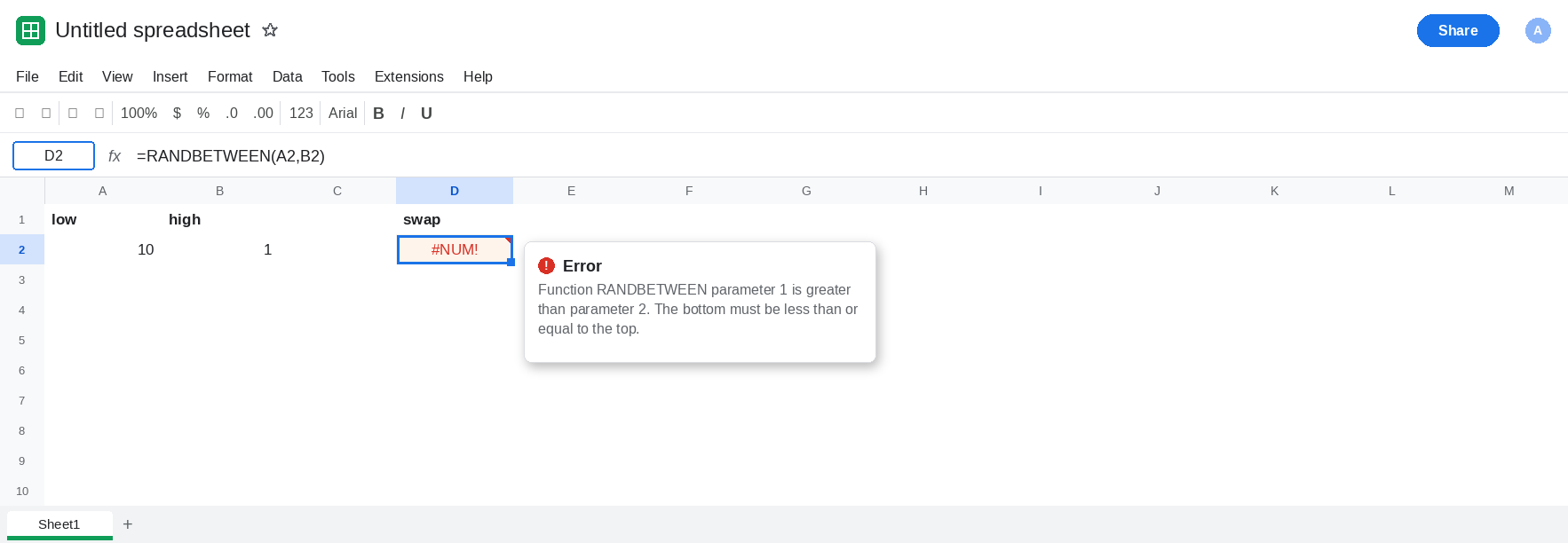
1. Open a blank spreadsheet. In A1 type low. A2 10. In B1 type high. B2 1. The labels say low and high. The numbers are backwards: 10 then 1.

Bottom greater than top. In D1 type swap. In D2 enter =RANDBETWEEN(A2,B2). The cell shows #NUM!. The tooltip names the parameter and says the first value has to be less than or equal to the second. A2 is 10. B2 is 1. Leave D2 broken.

The same numbers in order. In D4 type ok. In D5 enter =RANDBETWEEN(B2,A2). B2 is 1, A2 is 10. D5 is an integer from 1 through 10. Edit an empty cell, E1, type x, then delete it. D5 changes. D2 stays #NUM!. The working call is volatile. The broken call does not become a number just because the sheet recalculated. Leave D5 as a live integer. Leave D2 as #NUM!.

Equal ends. In D7 enter =RANDBETWEEN(4,4). D7 is 4. Bottom may equal top. The forbidden case is bottom greater than top, not a range of one integer.

Decimals truncate before the draw. In D9 enter =RANDBETWEEN(1.2,1.8). Both ends truncate to 1. The cell is 1 every time, including after an edit. It is not a random value between 1.2 and 1.8, and it is not #NUM!. There is no fractional result. Leave D9 as 1.

Constants, so the formula bar shows the order. In D11 enter =RANDBETWEEN(10,1). D11 is #NUM!, the same failure as D2, without cell references. Leave D11 broken.

Leave D2 and D11 as #NUM!. Leave D5 as an integer from 1 to 10. Leave D9 as 1.

What is actually wrong

• Argument order is the contract. First is the low end. Second is the high end. A2 and B2 are labeled as if the columns could absorb the swap. They cannot. D2 reads A2 first because you passed A2 first.
• Truncation happens first, toward zero. 1.2 becomes 1, 1.8 becomes 1, and RANDBETWEEN(1,1) is legal. D9. RANDBETWEEN(2.9, 2.1) truncates to RANDBETWEEN(2, 2) and returns 2. It does not become #NUM! just because 2.9 was typed before 2.1. Compare the integers after truncation when a decimal pair surprises you.
• Volatility is independent of #NUM!. D5 moves on unrelated edits. D2 does not start working on those edits. The storm page is RAND recalc storm. Do not rebuild it here.
• RAND() is a decimal from 0 inclusive to 1 exclusive. It has no bottom and top. RANDBETWEEN is the integer form. Mixing them up does not produce this #NUM!.
• A blocked RANDARRAY is #REF!, not #NUM!. See RANDARRAY spill. D2’s formula does not spill.

Other #NUM! domains, such as a negative argument to SQRT, are out of domain. This one is specifically the two ends of RANDBETWEEN.

Fix

Leave D2 as #NUM! with A2 still 10 and B2 still 1, so the swapped inputs stay visible.

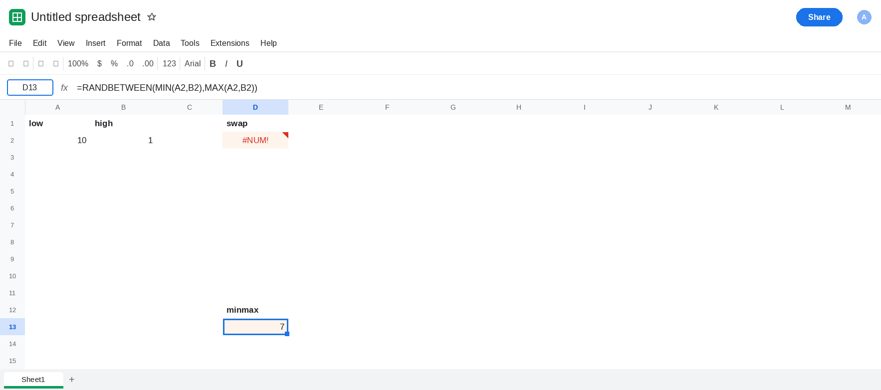
Put the smaller end first. In D13 enter =RANDBETWEEN(MIN(A2,B2),MAX(A2,B2)). The cell is an integer from 1 through 10, whichever cell is which. MIN and MAX absorb a labeled pair that might be typed backwards. Use this when the ends come from cells. When you are typing constants, write the low end first: =RANDBETWEEN(1,10).

Integers, if you meant integers. Keep D9 as the warning that 1.2 and 1.8 collapse to 1. Pass 1 and 2 when you want both. For a decimal between two limits, scale RAND(): =1.2+(1.8-1.2)*RAND(). That is a different function, and it is still volatile.

Do not wrap D2 in IFERROR and substitute 0. A zero hides the swapped range and looks like a real draw. See IFERROR vs IFNA.

If RANDBETWEEN is #NUM!, the first argument is greater than the second after truncation. Swap them, or take MIN and MAX. If the result is always the same integer, the two ends truncated to that integer. If a legal result changes on every edit, the formula is volatile, and that behavior is the recalc page.