Fix REGEXEXTRACT #N/A in Google Sheets (pattern did not match)

REGEXEXTRACT returns #N/A when the regular expression does not match the text. The formula ran. There was nothing to extract. That is the same error value as a lookup miss. It is not a missing sku and not a FILTER with zero rows.

This page is regex no match. It is not what #N/A means (VLOOKUP / MATCH / FILTER), not VLOOKUP no match (number vs text, or a trailing space), and not FILTER no match.

Recreate it on a blank sheet

1. Open a blank spreadsheet. In A1 type text, B1 extract, C1 match.
2. In A2 type SKU-101. In B2 enter =REGEXEXTRACT(A2,"SKU-(\d+)"). The cell shows 101. That row is the control: the pattern matches, the capturing group has digits.
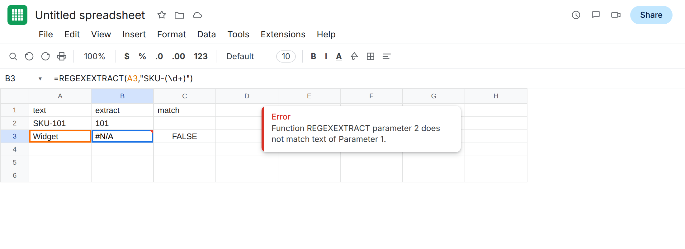
3. In A3 type Widget. In B3 enter =REGEXEXTRACT(A3,"SKU-(\d+)"). The cell shows #N/A. There is no SKU- and no digits. The pattern does not match.

REGEXMATCH on the same miss. In C3 enter =REGEXMATCH(A3,"SKU-(\d+)"). The cell shows FALSE. Same text, same pattern. REGEXMATCH does not use #N/A for “no match.” REGEXEXTRACT does.

B3 selected. Formula bar shows =REGEXEXTRACT(A3,"SKU-(\d+)"). B3 is #N/A. C3 is FALSE. A3 is Widget. B2 is 101 from SKU-101.

Capturing nothing. In A4 type SKU- with the hyphen and no digits after it. In B4 enter =REGEXEXTRACT(A4,"SKU-(\d+)"). The cell shows #N/A. You can see the prefix. The capturing group (\d+) still captured nothing, so the whole pattern fails. Same error value as Widget.

B4 selected. Formula bar shows =REGEXEXTRACT(A4,"SKU-(\d+)"). A4 is SKU-. B4 is #N/A. B3 is still #N/A. C3 is FALSE.

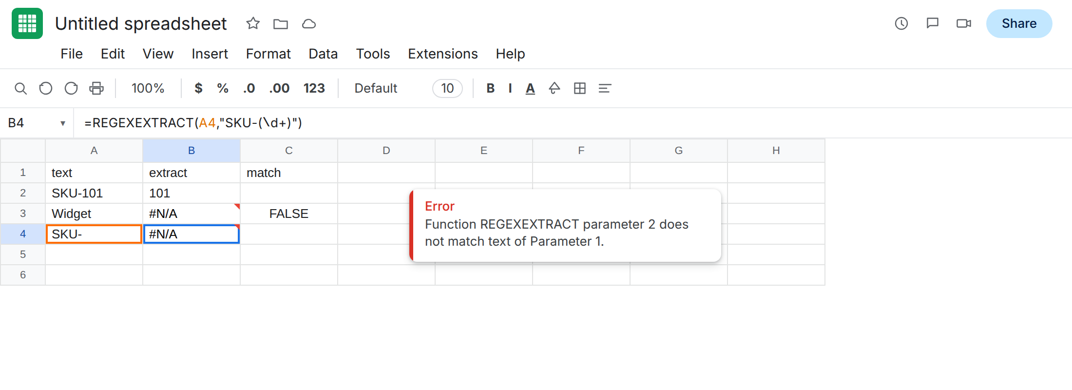
Leave B3 and B4 as the broken formulas.

What is actually wrong

• REGEXEXTRACT needs the pattern to match. Widget does not contain SKU- followed by digits. Sheets returns #N/A, not a blank.
• A prefix you can see is not enough. SKU- matches the literal part. (\d+) needs one or more digits. None are there, so the extract is still #N/A. That is capturing nothing — still a failed match, not a blank cell.
• Parentheses change what is returned. With SKU-(\d+), a hit returns only the digits (101), not the whole SKU-101. If that group cannot match, you get #N/A, not an empty string.
• REGEXMATCH on the same miss is FALSE. Do not debug C3 as #N/A. If the cell is #N/A, you are looking at REGEXEXTRACT (or a lookup), not a REGEXMATCH no-match.
• A pattern that is allowed to capture empty text is a different result. =REGEXEXTRACT(A4,"SKU-(.*)") returns a blank, because (.*) matches zero characters. (\d+) cannot. Blank vs #N/A is the quantifier, not a different error family.
• REGEXREPLACE on a miss returns the original text unchanged. It is not #N/A. This page is extract / match.

This is not a VLOOKUP key miss. Nothing is being looked up. See what #N/A means.

This is not number vs text in a lookup column. See VLOOKUP no match.

This is not FILTER with zero rows or mismatched heights. See FILTER no match.

This is not #VALUE!. A number in the text argument (=REGEXEXTRACT(101,"\d+")) is #VALUE! because regex functions want text. See wrong type. Convert with TEXT if you meant to extract from a numeric cell. B3 is already text.

This is not #REF! from a broken pattern. An invalid regular expression is #REF!, not #N/A. The patterns on this sheet are valid RE2. The text did not match.

Fix

Leave B3 and B4 as the broken extracts so #N/A stays on the sheet.

Confirm the miss. In A3 type SKU-101. B3 becomes 101. Put Widget back. If changing the text makes #N/A come and go, the function is working and the pattern does not match that row.

Fix the pattern when the text is right. If A3 is supposed to be a sku code and is Widget, that row has no sku to extract — do not rewrite the regex to silence it. If A4 should have been SKU-101 and someone omitted the digits, type the digits. B4 becomes 101.

When no match is a valid result. Then wrap. In B6 enter =IFNA(REGEXEXTRACT(A3,"SKU-(\d+)"),"none"). The cell shows none. In B7 enter =IFNA(REGEXEXTRACT(A4,"SKU-(\d+)"),"none"). The cell shows none.

B6 selected. Formula bar shows =IFNA(REGEXEXTRACT(A3,"SKU-(\d+)"),"none"). B6 and B7 are none. B3 and B4 are still #N/A.

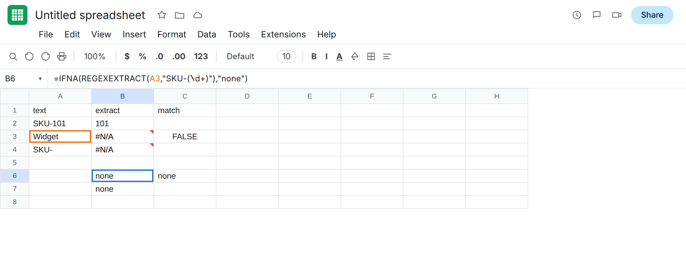
Use IFNA, not IFERROR. IFNA catches only #N/A. IFERROR also swallows #VALUE! from a numeric input and #REF! from a broken regex, so those look like “none.” See IFERROR vs IFNA.

Test with REGEXMATCH before you extract. In C6 enter =IF(REGEXMATCH(A3,"SKU-(\d+)"),REGEXEXTRACT(A3,"SKU-(\d+)"),"none"). The cell shows none. FALSE is the miss. You do not wrap REGEXMATCH in IFNA.

Do not wrap a miss you have not confirmed. If A2 is SKU-101 and B2 is #N/A, the pattern is wrong (a missing hyphen, a letter class where you needed digits, an extra ^ that requires the match at the start). Fix the pattern. IFNA will not.