Fix TEXT #VALUE! in Google Sheets (bad format code or a non-numeric input)

TEXT(number, format) turns a number, date, or time into text using a pattern. #VALUE! means the pattern is illegal, or the first argument is not a number Sheets can format. A legal pattern on a real date returns text that looks like a date and will not add. That second outcome has no red triangle. It is still the wrong type if the next formula expects a date serial.

This page is TEXT format codes on an English / United States locale sheet. It is not VALUE() locale (text into a number). It is not TO_PURE_NUMBER (strip a currency format off a number). It is not DATEVALUE locale. Keep the Google Sheets UI in English.

Recreate it on a blank sheet

1. Open a blank spreadsheet. Confirm File → Settings → Locale is United States for this recreate, so the decimal mark in a format is . and the thousands mark is ,. In A1 type n. A2 1234.5 as a number. In A4 type label. A5 pcs as text. In A7 type shipped. In A8 enter =DATE(2024,1,15).

A format that works. In C1 type ok. In C2 enter =TEXT(A2,"$#,##0.00"). The cell shows $1,234.50. It is text. =ISTEXT(C2) is TRUE. That row is the control.

Text input. In C4 type text_in. In C5 enter =TEXT(A5,"0.00"). The cell shows #VALUE!. pcs is not a number, date, or time. A format cannot invent a quantity. Leave C5 broken.

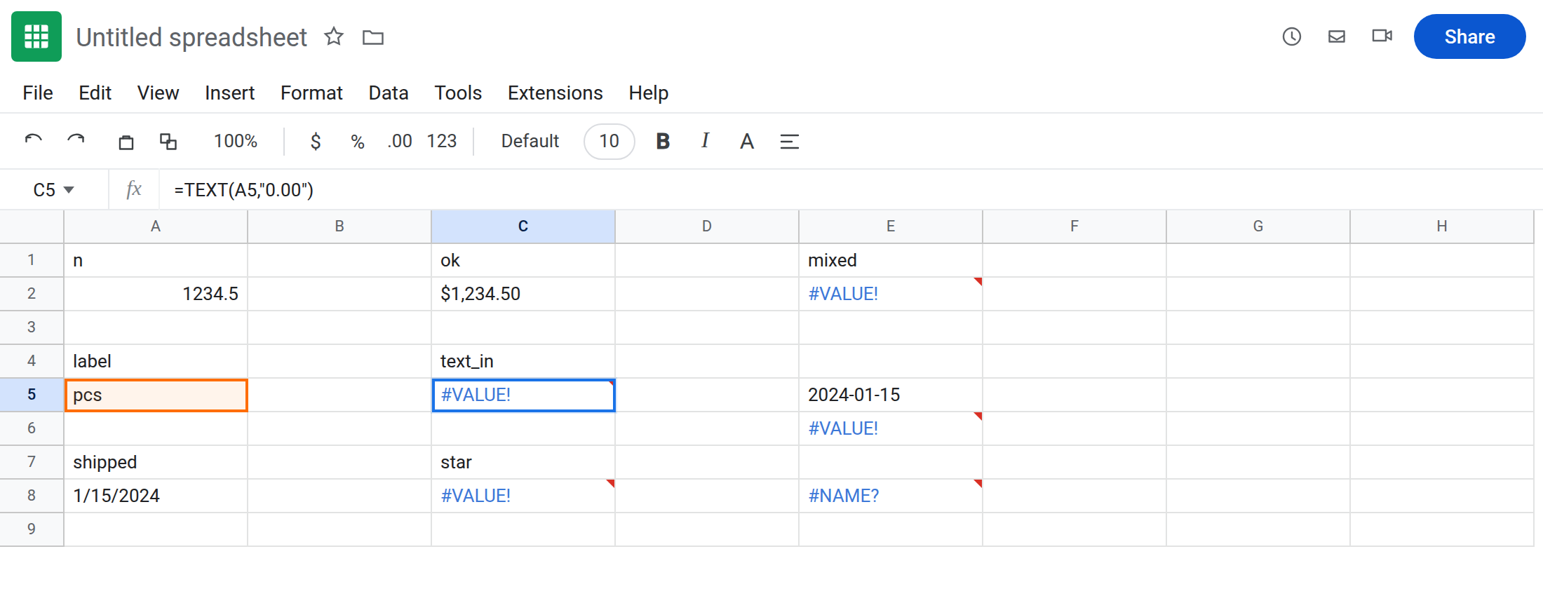
Asterisk in the pattern. In C7 type star. In C8 enter =TEXT(A2,"0.00*"). The cell shows #VALUE!. The tooltip names an invalid format pattern. Google Sheets does not allow * in a TEXT format (Excel uses * as a fill character). Leave C8 broken.

Date pattern mixed with a number pattern. In E1 type mixed. In E2 enter =TEXT(A8,"yyyy-mm-dd 0"). The cell shows #VALUE!. Date and time codes cannot share a pattern with 0 or #. The trailing 0 was meant as a literal. It is a number code. Leave E2 broken.

A date pattern that works, and then breaks addition. In E5 enter =TEXT(A8,"yyyy-mm-dd"). The cell shows 2024-01-15 with no error triangle. In E6 enter =E5+1. E6 shows #VALUE!. E5 is text. Adding 1 is wrong type. The format itself was legal. Leave E6 broken so the cascade stays visible. Leave E5 as the text date.

Unquoted pattern, for contrast. In E8 enter =TEXT(A8,yyyy-mm-dd). The cell shows #NAME? or a Formula parse error, not C5’s #VALUE!. yyyy is read as a name because it is not inside quotes. See unknown function if the tooltip is Unknown function or an unknown name. Leave E8 as that contrast.

Leave C5, C8, E2, and E6 broken. Leave C2 and E5 as successful TEXT results.

What is actually wrong

• The second argument is a pattern, not an example of the output. "0.00" means two decimal places. "pcs" as the input is not a pattern problem. C5 fails before the pattern matters.
• * is forbidden in the format. ? as a digit placeholder is an Excel pattern Sheets does not support. Do not copy ** fill codes or ? digit slots from an Excel format dialog.
• Date/time tokens (yyyy, mm, dd, hh, ss, AM/PM) and number tokens (0, #) cannot be combined in one pattern. E2. A literal character that is not a code can sit in quotes inside the pattern, but a bare 0 is always a digit code.
• On a United States locale, . is the decimal mark inside the format string and , is thousands. A pattern copied from a comma-decimal locale, such as "0,00", does not mean “two decimal places” here. It often returns a string with no error triangle and the wrong shape. That is a locale format, not C8’s invalid pattern. Do not change File → Settings locale just to make one TEXT call match a foreign pattern — that also changes argument separators for every formula. See locale parse error only when the formula itself shows Formula parse error.
• TEXT output is text even when it looks like $1,234.50 or 2024-01-15. ISTEXT is TRUE. Later math is #VALUE!. Format the cell (Format → Number) when you still need a number. Use TEXT when a label, a file name, or a QUERY date literal needs a string.

This is not VALUE("1.234,56") on a US sheet. See VALUE() locale. VALUE parses text. TEXT writes text.

This is not TO_PURE_NUMBER of a currency-formatted number. See TO_PURE_NUMBER. That function does not take a format code.

This is not DATEVALUE of 13/1/2024. See DATEVALUE locale. C5’s input is pcs, not a date string.

Fix

Leave C5, C8, E2, and E6 broken.

Format a number with a legal pattern. Keep C2: =TEXT(A2,"$#,##0.00"). For the ship date, keep E5: =TEXT(A8,"yyyy-mm-dd"). Month names are "mmm" or "mmmm", not the letters Jan as a code (some three-letter strings are treated as literal text and some patterns error — use the m codes).

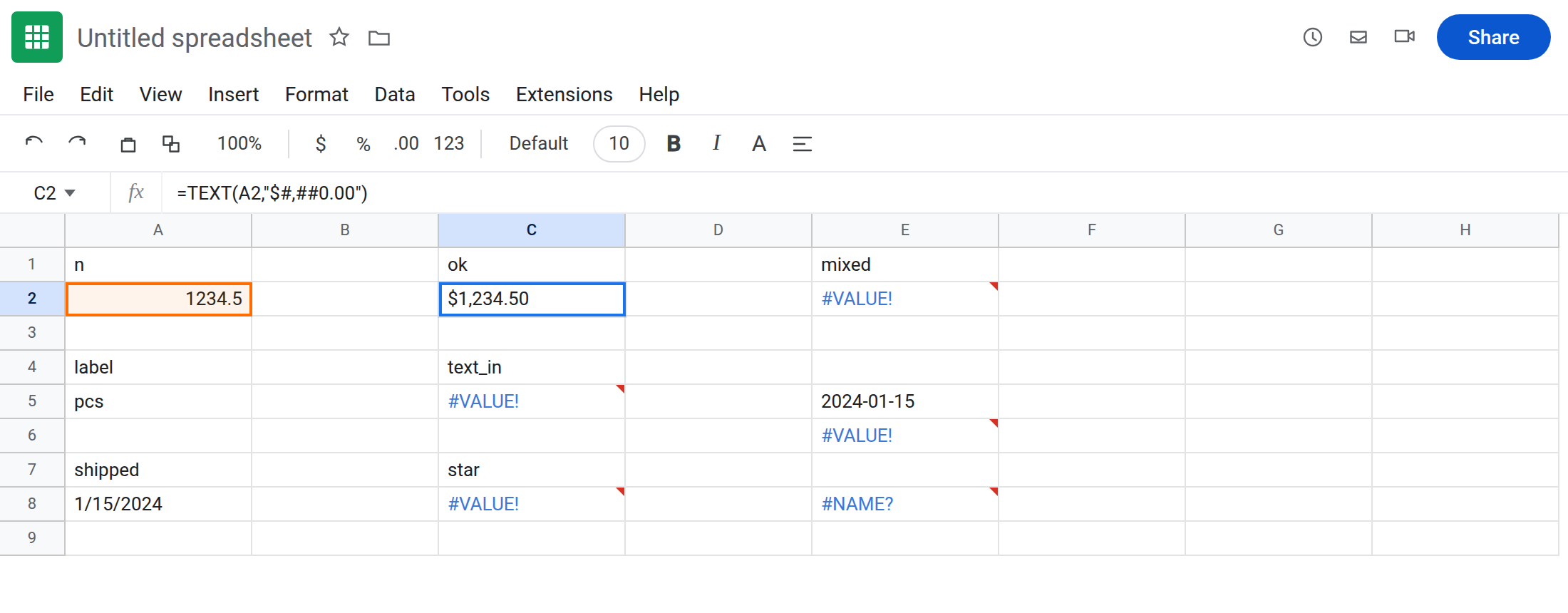
If the input might be text, test it: =IF(ISNUMBER(A5),TEXT(A5,"0.00"),""). pcs becomes blank instead of #VALUE!. Do not wrap C8 in IFERROR — the pattern is still illegal on every row.

If you need math, do not add the TEXT result. Add A2 or A8, and format those cells. E6 is the reason.

A literal in the pattern that would otherwise be a code can be quoted inside the format string: =TEXT(A8,"yyyy-mm-dd"" dock""") produces a text label ending in dock. The doubled quotes are how a quote sits inside a quoted format. They are not the * problem.

If TEXT is #VALUE!, check the first argument with ISNUMBER and check the pattern for *, ?, or a mix of date codes and 0/#. If there is no triangle and the next cell is #VALUE! on +, the format already succeeded and the result is text.