MODE.MULT spills every mode and #REF! when the next cell is filled

MODE.MULT(range) returns every value that is tied for the highest frequency. One mode is one cell. Two modes are a vertical spill. If the cell under the formula already has a value, the spill cannot expand and the formula cell shows #REF!. The tooltip says the array result was not expanded because it would overwrite data. MODE.SNGL returns a single mode and does not need that extra row. If nothing repeats, both functions return #N/A.

A blocked spill is the same family as SORT / UNIQUE spill. #N/A as “no match” in a lookup is what #N/A means. Keep the Google Sheets UI in English. Sheet Error is an independent formula-error library, not a Google product.

Recreate it on a blank sheet

1. Open a blank spreadsheet. In A1 type n. A2 4. A3 4. A4 7. A5 7. A6 1. A7 9. Six numbers. 4 appears twice. 7 appears twice. 1 and 9 appear once. There are two modes.

A clear spill. In C1 type mult. In C2 enter =MODE.MULT(A2:A7). C2 and C3 fill with 4 and 7, in whichever order Sheets lists the tie. Two cells, both modes, no triangle. That block is the control: the rows under the formula were empty.

Block the spill. In C3 type note. You just wrote into the second row of the result. C2 changes to #REF!. The tooltip is that the array was not expanded because it would overwrite C3. note is still in C3. The modes did not become “invalid.” They have nowhere to land. Leave C2 as #REF! and leave note in C3.

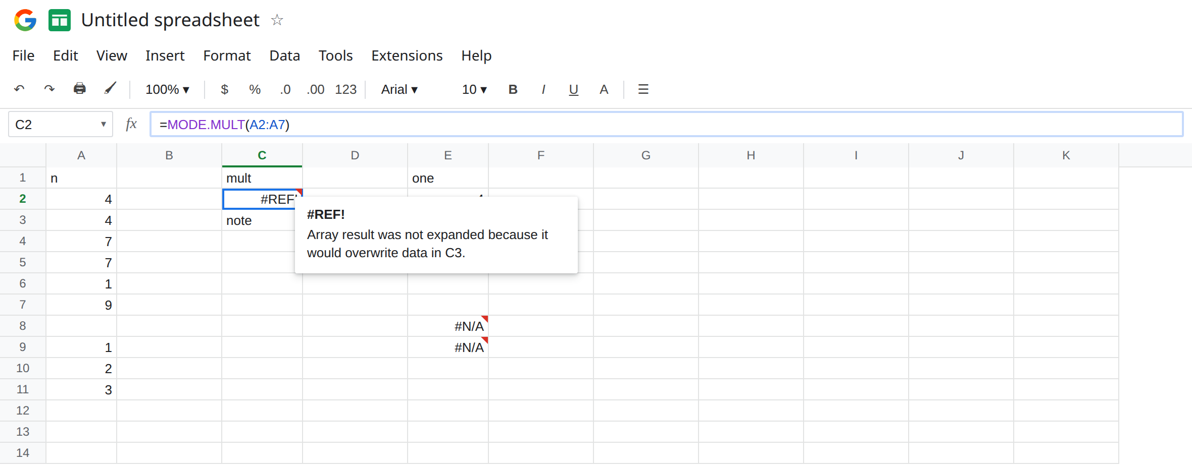
One mode does not need the second row. In E1 type one. Change nothing in column A yet. In E2 enter =MODE.MULT(A2:A3). Only the two 4s. E2 is 4. E3 stays empty. A single mode does not collide with a neighbor below. The #REF! in C2 needs the tie.

MODE.SNGL. In E5 enter =MODE.SNGL(A2:A7). E5 is one number, either 4 or 7. It does not spill. It also does not tell you there was another mode. If the spec is “list every mode,” MODE.SNGL is the wrong function even when it shows no error. The older MODE is the single-mode function as well.

Nothing repeats. In A9 type 1, A10 2, A11 3. In E8 enter =MODE.MULT(A9:A11). E8 is #N/A. In E9 enter =MODE.SNGL(A9:A11). E9 is #N/A. No value appears more than the others, so there is no mode. That #N/A is not the overwrite in C2. Move note and C2 still would not fix E8.

Leave C2 as #REF!. Leave E8 as #N/A. Leave the clear one-mode result in E2 as 4.

What is actually wrong

• MODE.MULT is an array. The height is “how many values share the winning frequency,” not a height you pass in. Two winners need two rows. Three winners need three. A note, a header, or another formula in that strip is #REF!.
• The overwrite tooltip names the blocked cell. Here it is C3. Clearing C4 does nothing if C3 is the one in the way. The same rule as UNIQUE: only the occupied cell inside the spill matters. See UNIQUE spill.
• MODE.SNGL hides the tie. A chart title that says “the mode” next to E5 is incomplete when C2’s spill, once it has room, shows two numbers.
• All frequencies equal to 1 is #N/A, not 0 and not blank. IFERROR(E8,0) would invent a mode of 0 that is not in A9:A11. The data has no mode.
• Text in the range is ignored for the frequency count. A column of labels plus two numeric 4s still has a mode of 4. Blank cells are ignored. They do not create a blank mode.
• MODE.MULT of a single cell, or of an empty range, is #N/A. There is no frequency to compare.

This is not SORTN tie mode. See SORTN ties mode. That function returns rows from a table, not the modal number.

This is not #VALUE! from a bad argument count. The formula in C2 parsed. The spill collided.

Fix

Leave C3 as note so C2 stays #REF!. Leave E8 as #N/A.

Give the spill empty rows, or move the formula. In G1 type mult_ok. In G2 enter =MODE.MULT(A2:A7). G2 and G3 show 4 and 7. Nothing sits under G2. If you need the note, put it in G5, below a spill you know is only two rows, or put it in column I.

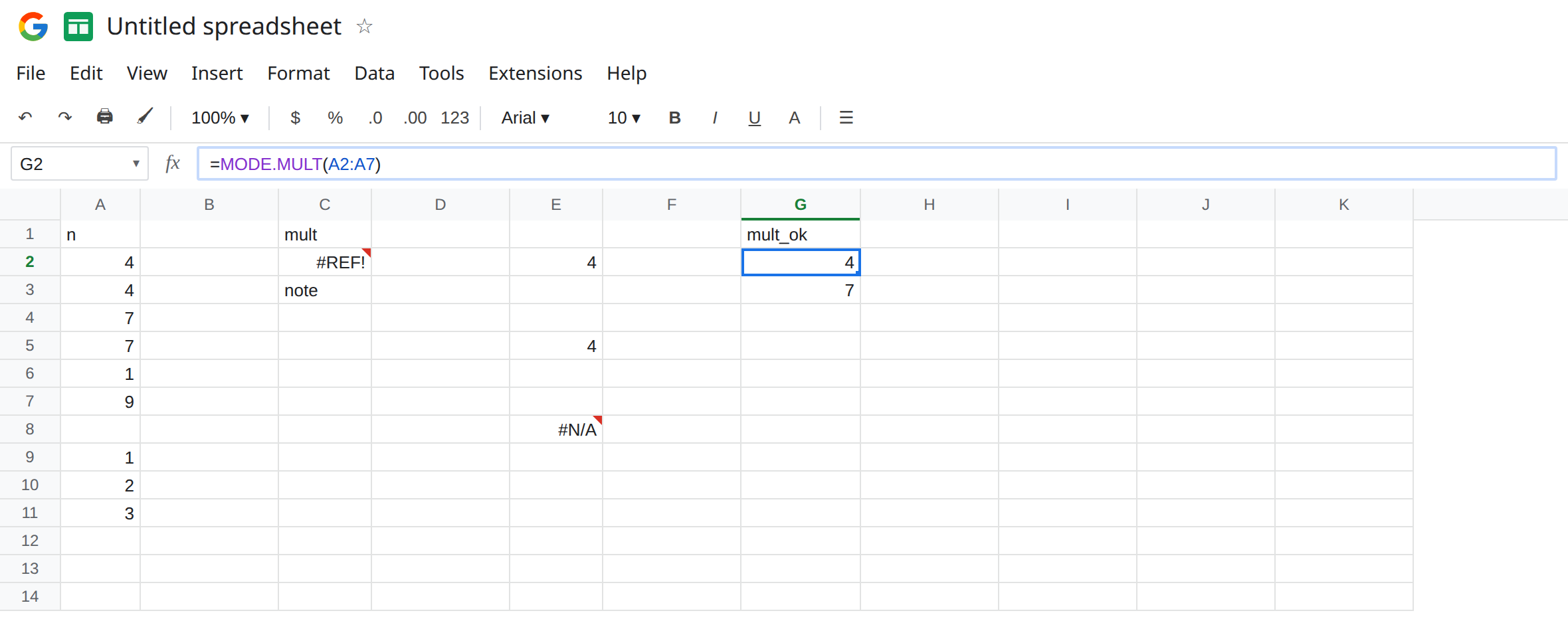
If you only want one mode, call MODE.SNGL and accept that a tie is silent. E5 already does that. Do not point MODE.SNGL at a blocked MODE.MULT cell and expect it to list both.

If #N/A and the values really are all unique, the function is right. Report “no mode” with =IFNA(MODE.MULT(A9:A11),"no mode"). IFNA fits because this failure is #N/A. Do not use IFNA on C2. C2 is #REF!. See IFERROR vs IFNA.

If MODE.MULT is #REF!, clear the cells under it until the modes appear, or move the formula. If it is #N/A, nothing repeats. If MODE.SNGL shows one number and you needed every tie, switch to MODE.MULT and leave room for the spill.

Spill vs single vs no mode

C2 is #REF! because two modes want C2:C3 and C3 says note. G2 is the same formula with room. E2 is one mode and uses one cell. E5 is MODE.SNGL and never lists the second mode. E8 is #N/A because 1, 2, and 3 never repeat. Clearing C3 does not change E8.