MINIFS and MAXIFS return 0 when nothing matches

MINIFS(range, criteria_range1, criterion1, …) and MAXIFS return the smallest or largest number on rows that pass. If no row passes, both functions return 0. They do not return blank, and they do not return #N/A. A region whose quantities are actually zero looks the same as a region that is not on the sheet. The cell has no triangle either way.

A criteria range that is a different size is a different failure: #VALUE!. That recreate is MAXIFS / MINIFS size. An average of no numbers is #DIV/0!, not 0. That is AVERAGEIF #DIV/0!. Keep the Google Sheets UI in English. Sheet Error is an independent formula-error library, not a Google product.

Recreate it on a blank sheet

1. Open a blank spreadsheet. In A1 type region, B1 qty. A2 East, B2 10. A3 East, B3 0. A4 West, B4 20. Three data rows. East’s quantities are 10 and a real zero.

Real zero. In D1 type min_east. In D2 enter =MINIFS(B2:B4,A2:A4,"East"). D2 is 0. That zero is the cell B3. It is a successful minimum. In D3 enter =MAXIFS(B2:B4,A2:A4,"East"). D3 is 10. East exists. The max proves the group is on the sheet even though the min is 0.

No such region. In F1 type min_north. In F2 enter =MINIFS(B2:B4,A2:A4,"North"). F2 is 0. In F3 enter =MAXIFS(B2:B4,A2:A4,"North"). F3 is 0. North is not in column A. Both the min and the max are 0. Nothing in the tooltip says “no match.” If you only glance at F2, it is identical to D2.

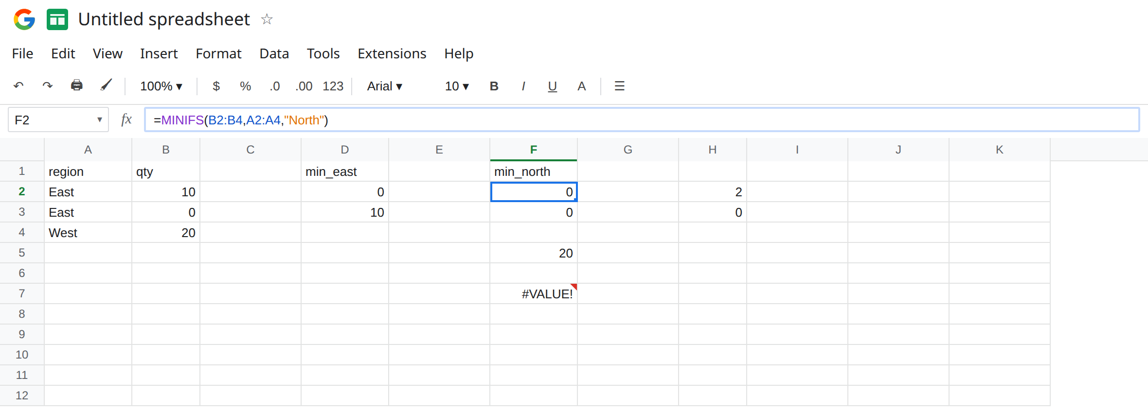
Count the rows. In H2 enter =COUNTIFS(A2:A4,"East"). H2 is 2. In H3 enter =COUNTIFS(A2:A4,"North"). H3 is 0. The mins matched. The counts did not. H3 is how you tell F2 from D2.

A West minimum that is not zero. In F5 enter =MINIFS(B2:B4,A2:A4,"West"). F5 is 20. A group can have a non-zero min. The ambiguous case is only when the function returns 0.

Size error, so you do not confuse it with this zero. In F7 enter =MINIFS(B2:B4,A2:A5,"East"). Four criteria rows, three quantities. #VALUE!. Tooltip: Array arguments to MINIFS are of different size. That is MAXIFS / MINIFS size. Leave F7 broken. Do not “fix” F2 by adding a row to the range.

Leave F2 and F3 as 0. Leave D2 as the real 0. Leave H3 as 0 rows.

What is actually wrong

• Google Sheets documents this: if none of the criteria are satisfied, MINIFS returns 0. MAXIFS does the same. The 0 is a number. IF(F2=0,"missing",F2) is true for North and for East. The test cannot see B3.
• A blank criteria cell is not a match for "North". It also does not turn the result into blank. No pass still means 0.
• Text in the min range is ignored. If East’s only special cell were the word TBD and you had no numeric East row, you are in the “no numeric match” case and the result is still 0, not #VALUE! and not #DIV/0!. AVERAGEIFS of that row is #DIV/0!. Do not copy an average guard onto MINIFS and expect the same error value.
• MIN of B2:B4, with no criteria, is 0 because B3 is in the range. MIN does not know about North. Switching from MINIFS to MIN to “avoid the zero” drops the criterion and still shows 0.
• Same-size ranges that start on different rows can return 0 because the zipped pairs never see East. That zero is a window bug. The sizes match, so there is no #VALUE!. Check the start row before you conclude the region is missing. H2 counts the region in the same window you passed to MINIFS.

This is not a lookup #N/A. VLOOKUP of North would be #N/A. MINIFS refuses to use that token. See what #N/A means.

This is not IFERROR. There is no error to catch. Wrapping F2 hides nothing and changes nothing, because 0 is a normal result. See IFERROR vs IFNA.

Fix

Leave F2, F3, and D2 as the two zeros. Leave F7 as #VALUE!.

Ask COUNTIFS before you trust a zero. In J2 enter =IF(COUNTIFS(A2:A4,"East")=0,"no match",MINIFS(B2:B4,A2:A4,"East")). J2 is 0, and this time the 0 is allowed, because H2 is 2. In J3 enter =IF(COUNTIFS(A2:A4,"North")=0,"no match",MINIFS(B2:B4,A2:A4,"North")). J3 is no match. Use the same criteria, in the same order, in both functions. A count range that is taller than the min range is #VALUE! inside the IF and you are back on the size page.

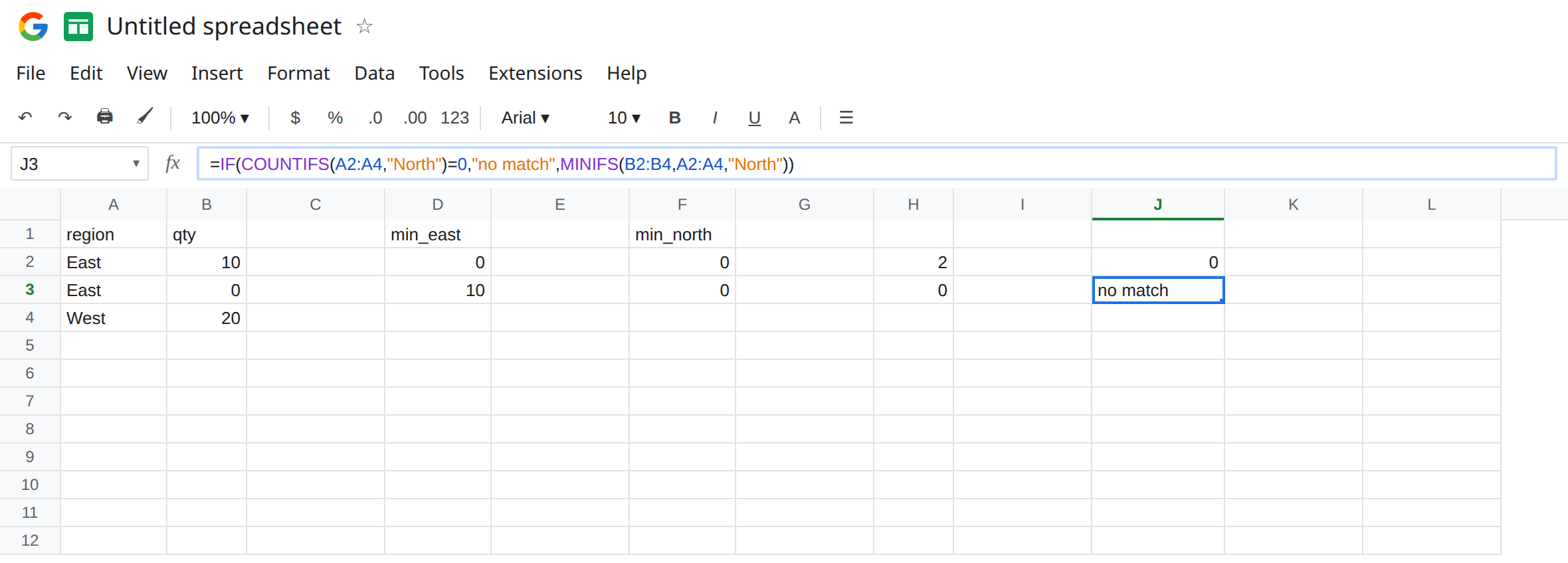
Do the same for MAXIFS. =IF(COUNTIFS(A2:A4,"North")=0,"no match",MAXIFS(B2:B4,A2:A4,"North")) is no match. F3 alone cannot say that. D3 stays 10 for East, so you do not need the label when the max is already non-zero — the label still matters the day the true max is 0.

Keep the ranges aligned with MAXIFS / MINIFS size before you interpret a zero. F7 is not a missing region.

If min and max are both 0 and COUNTIFS of the same criteria is 0, the group is absent (North). If the min is 0 and the count is greater than 0, a row really holds zero (East, B3). If the cell is #VALUE! and the tooltip says different size, fix the ranges. Do not replace that #VALUE! with 0.

Real zero vs no match vs size

D2 is 0 and H2 is 2: the minimum is zero. F2 is 0 and H3 is 0: nothing matched, and MAXIFS in F3 agrees by also showing 0. F7 is #VALUE!. AVERAGEIFS of North would be #DIV/0! instead of 0. Read the function name before you treat every zero as missing stock.