Fix VLOOKUP #N/A in Google Sheets (spaces and numbers stored as text)

You can see the lookup value with your eyes and VLOOKUP still returns #N/A. That is usually not a missing row. It is a key that does not actually match. FALSE exact match compares values, not what the cell looks like. Number vs text, and a trailing space, are the two recreates on this page.

If the sku is not in the column at all, start at what #N/A means. If the name sits left of sku, that is lookup left of the key. If File → Import produced the type split, that is CSV text vs number.

Recreate it on a blank sheet

1. Open a blank spreadsheet. In A1 type sku, B1 name, D1 lookup, E1 result.
2. In A2 type 101 as a number. B2 Widget. In D2 type an apostrophe then 101 so Sheets stores it as text. In E2 enter =VLOOKUP(D2,A2:B2,2,FALSE). The cell shows #N/A.

E2 selected. Formula bar shows =VLOOKUP(D2,A2,2,FALSE). E2 is #N/A because A2 is numeric 101 and D2 is text 101.

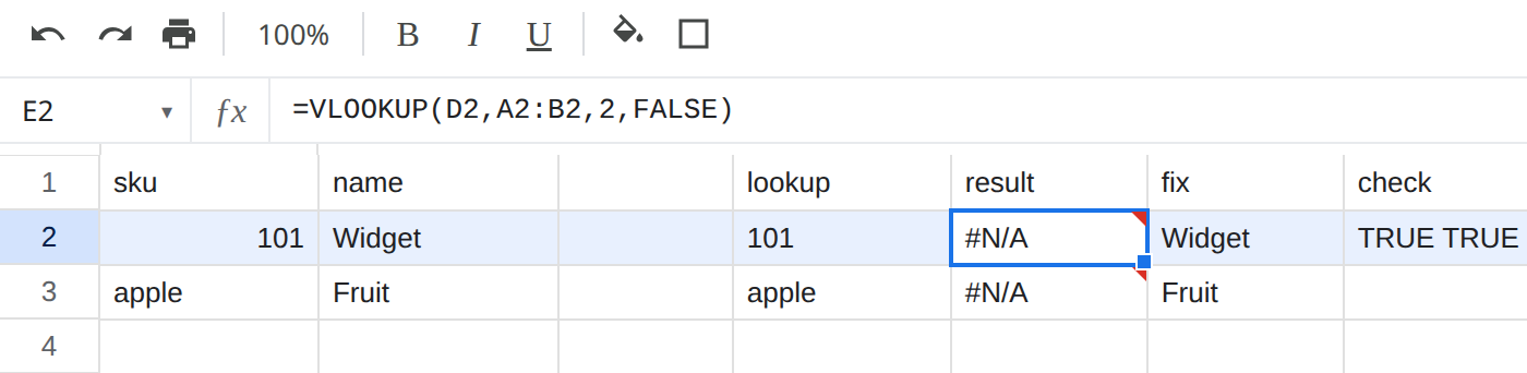
Leave E2 as the broken formula.

3. In A3 type apple then a space. B3 Fruit. D3 apple with no space. In E3 enter the same VLOOKUP against A3:B3. That cell is also #N/A.

E3 selected. Formula bar shows =VLOOKUP(D3,A3,2,FALSE). E3 is #N/A because A3 has a trailing space.

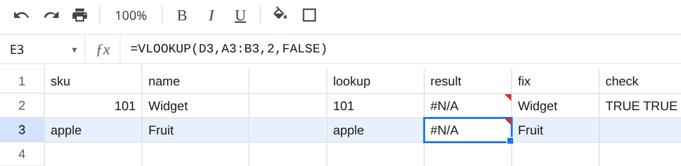
Leave E3 broken.

Check the keys, do not guess. In G1 type len_table, H1 len_lookup. In G3 enter =LEN(A3). The cell shows 6. In H3 enter =LEN(D3). The cell shows 5. In G2 enter =ISNUMBER(A2). TRUE. In H2 enter =ISTEXT(D2). TRUE. Same digits. Different types. Same word. Different lengths.

TRIM on the lookup only. In I1 type trim_lookup. In I3 enter =VLOOKUP(TRIM(D3),A3:B3,2,FALSE). The cell is still #N/A. D3 had no extra space. A3 did. Trimming the lookup cell cannot see a space that lives in the table.

What is actually wrong

Numbers and text are not the same key. 101 the number is not '101 the text. VLOOKUP with FALSE does not coerce them. The apostrophe is the reliable way to type a text number. Alignment is a hint (text left, numbers right) but ISNUMBER / ISTEXT is the check.

A trailing space in the table is a different string. apple is not apple . LEN is the check. TRIM on the lookup value only does not fix a space that lives in the table column.

This is not a missing sku. Widget and Fruit are on the sheet. Changing D2 to the number 101 (no apostrophe) makes E2 become Widget. Put the text '101 back so #N/A returns. That toggle is how you confirm type, the same way what #N/A means toggles 999 / 101 to confirm absence.

This is not lookup-left. The search column is A, and the key is meant to be in A. See lookup left of the key when the formula searches name for a sku.

This is not TRUE approximate match returning the wrong row. The fourth argument here is FALSE. The cell is #N/A, not a surprising name. See VLOOKUP wrong row.

This is not CHAR(160). A non-breaking space also looks like a normal key and also misses, but LEN is 4 on '101 plus CHAR(160), and TRIM stays 4. That cleanup is CHAR(160) blanks. Ordinary CHAR(32) space is this page: TRIM works once you point it at the table.

Fix

Leave E2 and E3 broken so #N/A stays on the sheet.

Number column: =VLOOKUP(VALUE(D2),A2:B2,2,FALSE) returns Widget. VALUE turns the text '101 into the number 101. If the table were text and the lookup a number, wrap the table key instead (VALUE on the first column, or TO_TEXT on the lookup). Do not wrap both and hope.

F2 selected. Formula bar shows =VLOOKUP(VALUE(D2),A2,2,FALSE) and F2 is Widget. Column E still shows #N/A. F3 is Fruit.

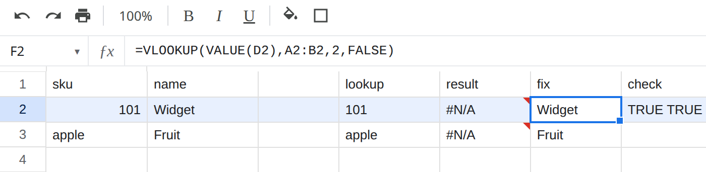
Space in the table: trim the table side, for example =VLOOKUP(D3,{TRIM(A3),B3},2,FALSE) returns Fruit. For real data, TRIM the sku column into a helper and lookup against that, not only the lookup cell. Inside { }, watch the locale column separator. See array literal locale.

If it looks equal and VLOOKUP disagrees, check type and LEN before you rewrite the formula. Do not wrap in IFNA until the keys actually match when the row should exist. See IFERROR vs IFNA.