DATEDIF units MD, YM, and YD are not leftover calendar days

DATEDIF(start_date, end_date, unit) has six unit strings. "Y", "M", and "D" are whole years, whole months, and days. "YM" is whole months after the years are removed. "MD" is days after the whole months are removed. "YD" is days between the dates as if they sat in the same year. The start must be on or before the end. Reverse them and every unit is #NUM!, including "MD". "MD" on a month-end start can be a negative number, a zero, or a day count that does not match the calendar you count by hand. The order is legal and the cell is still not the number you wanted.

The reverse-order #NUM! primer, including a bad unit such as "W", is DATEDIF #NUM!. YEARFRAC basis codes are YEARFRAC basis. Keep the Google Sheets UI in English. Format result cells as Number. A day count formatted as Date looks like 1900. Sheet Error is an independent formula-error library, not a Google product.

Recreate it on a blank sheet

1. Open a blank spreadsheet. In A1 type start, B1 end. In A2 enter =DATE(2020,3,10). In B2 enter =DATE(2024,11,25). Format both as Date. Mid-month dates, so the leftover units are the ones you can check on a calendar.

The six units. In D1 type Y. In D2 enter =DATEDIF(A2,B2,"Y"). D2 is 4. In E1 type YM. In E2 enter =DATEDIF(A2,B2,"YM"). E2 is 8. March 10 to November 10 is eight months, and November 25 is past the 10th, so the month count does not wait. In F1 type MD. In F2 enter =DATEDIF(A2,B2,"MD"). F2 is 15 (the 10th through the 25th, after those eight months). In G1 type D. In G2 enter =DATEDIF(A2,B2,"D"). G2 is 1721. In H1 type YD. In H2 enter =DATEDIF(A2,B2,"YD"). H2 is 260. That is the span from March 10 to November 25 inside one year, not 1721. In I1 type M. In I2 enter =DATEDIF(A2,B2,"M"). I2 is 56 (4*12+8). Format D2:I2 as Number.

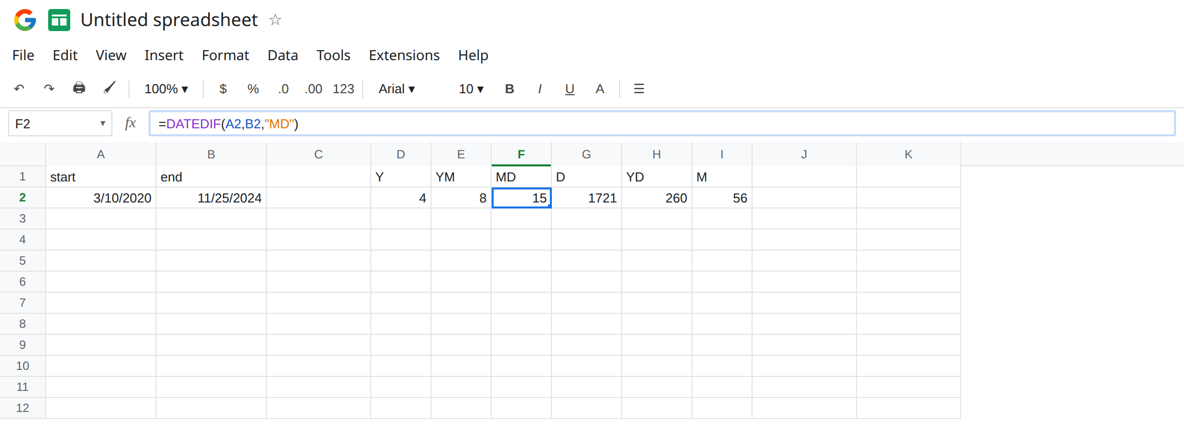
Age in three pieces. 4 years, 8 months, 15 days. Those three units are designed to be read together. "Y" plus "M" double-counts the years, because "M" is total months (56), not months after the last birthday. "YD" is not "Y" plus days. It throws the years away and keeps 260.

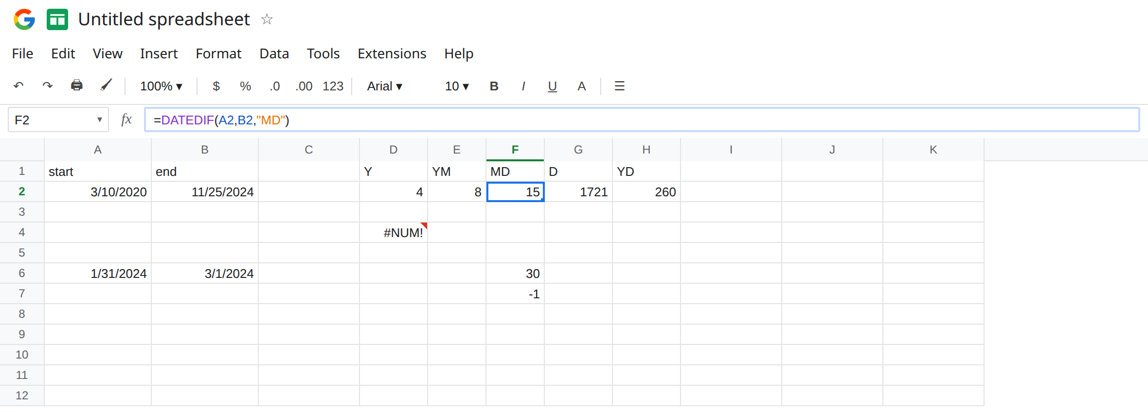
Reversed span. In D4 enter =DATEDIF(B2,A2,"MD"). End before start. D4 is #NUM!. In E4 enter =DATEDIF(B2,A2,"YM"). #NUM!. In H4 enter =DATEDIF(B2,A2,"YD"). #NUM!. The unit does not matter. The order does. Leave D4 broken. The full reverse-order recreate is DATEDIF #NUM!.

Month-end, where MD stops being obvious. In A6 enter =DATE(2024,1,31). In B6 enter =DATE(2024,3,1). In F6 enter =DATEDIF(A6,B6,"D"). F6 is 30. In F7 enter =DATEDIF(A6,B6,"MD"). Leave F7 as Sheets calculates it. If it is not the leftover you count on a calendar, or if it is negative, that is "MD". It may not be #NUM!. Do not replace F2’s 15 with F7.

Equal dates. In D8 enter =DATEDIF(A2,A2,"MD"). D8 is 0. Legal. Not #NUM!.

Leave D4 as #NUM!. Leave F2 as 15. Leave F7 visible.

What is actually wrong

• "MD" ignores months and years and keeps days. "YM" ignores days and years and keeps months, and it never goes past 11. "YD" ignores years and keeps days, and it is not D modulo 365. On this pair "YD" is 260 while "D" is 1721.
• "Y", "YM", and "MD" are the three-part age. Adding "Y" to "M" answers a different question (years, and also total months). Adding "MD" to "D" double-counts days.
• A negative or surprising "MD" with the earlier date first is the unit, not a corrupted workbook. Microsoft’s own notes on this inherited function say not to trust "MD". Google Sheets still accepts the string. Prefer "D" and DATE arithmetic when F7 disagrees with the calendar.
• Reversing the arguments is #NUM! for "MD" the same as for "D". A negative "MD" on a forward pair is not the same failure as D4. One has a triangle. The other may not.
• Formatting F2 as Date displays 15 as a date in January 1900. Format → Number → Number. That display bug is also on DATEDIF #NUM!.

This is not NETWORKDAYS. See NETWORKDAYS #NUM!. "YD" does not skip weekends.

This is not EOMONTH. See EOMONTH #NUM!. A6 is a real date.

Fix

Leave D4 and F7 as the two different failures (order, and "MD" on a month-end).

Use Y, YM, and MD only on the forward mid-month pair, and only as a set. Keep D2, E2, and F2. The age sentence is those three cells: 4, 8, and 15. For a single day count, keep G2: =DATEDIF(A2,B2,"D"), which is 1721. For days since the anniversary in the current year, H2 is 260, and the header should say that, not “total days.”

Unknown order. =IF(B2>=A2,DATEDIF(A2,B2,"D"),DATEDIF(B2,A2,"D")) is an unsigned day gap. See IFERROR vs IFNA.

Replace month-end MD. Days after the first of the end month are =B6-DATE(YEAR(B6),MONTH(B6),1). That expression does not use "MD". Use it when F7 looks wrong and the order is already forward.

Do not wrap D4 in IFNA. #NUM! is not #N/A.

If every unit is #NUM! and the later calendar date is in the first argument, swap them. If "D" is 1721 and "YD" is 260, both are right and they are different units. If "MD" is negative or strange and "D" looks right, stop using "MD". If the cell looks like a 1900 date, change the format to Number.

Units on 10 Mar 2020 → 25 Nov 2024

"Y" is 4. "YM" is 8. "MD" is 15. Together that is the age in parts. "M" is 56, not 8. "D" is 1721. "YD" is 260. Reversed arguments are #NUM! for "MD", "YM", and "YD". January 31 to March 1 is where "MD" stops matching a hand count. "W" is not a unit. See DATEDIF #NUM!.