CHOOSE of an array literal spills a different shape once ARRAYFORMULA is wrapped around it

CHOOSE(index, choice1, choice2, …) returns one of the choices by position. A choice can be an array literal, {1,2,3}. A scalar choice such as "Hold" returns one cell. A literal is several cells, and Sheets may show only the first number or spill the whole row. Wrapping the same call in ARRAYFORMULA changes that decision on many files: one version is a single 1, the other spills 1, 2, 3 into the cells beside it, or the spill hits a neighbor and becomes #REF!. The index did not change. The wrapper did. A range of indexes in that wrapper does not become “row 1 gets {1,2,3}, row 2 gets {4,5,6}.” CHOOSE does not spread a range into separate choices, and it does not map a column of indexes onto a pair of literals the way MAP maps a column of scalars.

Sheet Error is an independent formula-error library, not a Google product. An index of 0 or past the list is CHOOSE #VALUE! and CHOOSE index 0. A blocked spill’s tooltip is array result was not expanded. Brace separators on a comma-decimal locale are array literal locale. Keep the Google Sheets UI in English. File → Settings → Locale → United States for the braces in this recreate.

Recreate it on a blank sheet

1. Open a blank spreadsheet. Locale United States, so {1,2,3} uses commas. In A1 type idx. In A2 type 1. In A3 type 2.

Scalar choices, the control. In C1 type word. In C2 enter =CHOOSE(A2,"Open","Hold","Closed"). C2 is Open. ARRAYFORMULA around that one call does not add cells. One choice, one value.

The literal, no wrapper. Clear D2:F4. In D2 enter =CHOOSE(1,{1,2,3},{4,5,6}). Look at D2:F2. Either D2 is 1 and E2:F2 are empty, or D2:F2 spill 1, 2, 3. Write down which one you got. The second literal {4,5,6} is not selected, because the index is 1. If the cell is #ERROR! Formula parse error, the locale wanted a backslash inside the braces. See array literal locale. Fix the locale or the separator before you judge the spill.

The same call inside ARRAYFORMULA. Clear D5:F7. In D5 enter =ARRAYFORMULA(CHOOSE(1,{1,2,3},{4,5,6})). Compare D5:F5 to D2:F2. The bug is a difference. One row shows a lone 1. The other spills 1, 2, 3. If both rows spill the same three numbers, this file already returns the literal from CHOOSE and the wrapper did not change a constant index. Leave both formulas. The next step is the one that still fails.

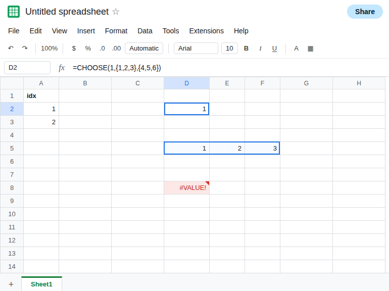
A column of indexes does not zip. In D8 enter =ARRAYFORMULA(CHOOSE(A2:A3,{1,2,3},{4,5,6})). You wanted two rows: 1,2,3 and then 4,5,6. What you get is one of these, and you should believe the grid: a single row from the first index, a #VALUE! or #N/A about the index, or a #REF! because the spill ran into D5. You do not get a clean two-by-three block that follows A2 and A3. Leave D8 as that result.

CHOOSE(A2, D2:F2, D5:F5) is a different mistake. A range is one argument, not a list of choices. The tooltip can say the index is valid only between 1 and 1, because both ranges collapsed into a single choice. That error is real. Adding ARRAYFORMULA does not split the range into three arguments.

What is actually wrong

• CHOOSE returns one argument. An array literal is one argument that happens to hold three numbers. Whether those three paint across the row depends on the formula engine and on ARRAYFORMULA. The help text that shows a single returned value does not mention the spill. Your two formulas are the test.
• ARRAYFORMULA does not mean “run CHOOSE once per row and spill that row’s literal.” The index A2:A3 is not applied as two separate positions against two literals. People who need that layout are asking for a per-row IF or for CHOOSECOLS on a real block.
• A range written as a choice is not expanded into arguments. There is no spread syntax. CHOOSECOLS and CHOOSEROWS exist for picking columns or rows out of a range. See CHOOSECOLS from right for the sign of those indexes. They are not CHOOSE.
• A spill that meets a typed cell is #REF!, Array result was not expanded. Clearing the literal’s neighbors is required before you decide the function returned one number on purpose. See array result was not expanded.
• Index 0 is still #VALUE! whether or not the choices are literals. See CHOOSE index 0.

Fix

Leave D2 and D5 as the pair that disagree, and leave D8 as the failed zip.

A constant index can return the literal without CHOOSE. In H2 enter ={1,2,3}. H2 spills 1, 2, 3 on a US locale if H3:I2 are empty. You do not need CHOOSE or ARRAYFORMULA when the index is the constant 1.

A single index cell can pick a literal with IF. In H5 enter =IF(A2=1,{1,2,3},{4,5,6}). With A2 as 1, H5 spills 1, 2, 3. Change A2 to 2 and the spill becomes 4, 5, 6. That is one row, one index. It is not D8.

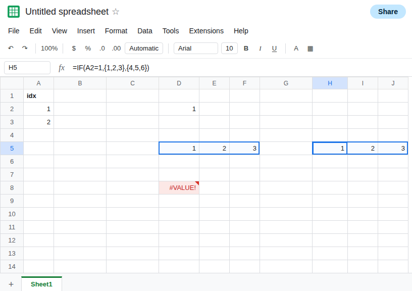
Two indexes, two formulas, or a real table. Put =IF(A2=1,{1,2,3},{4,5,6}) in H5 and the same pattern in H6 pointed at A3. Or store both literals as rows on the sheet and use INDEX or CHOOSEROWS. MAP that returns {1,2,3} from the lambda hits the nested-array error. See MAP nested return. Do not wrap that MAP in another ARRAYFORMULA and expect a rectangle.

Do not hide D8 with IFERROR. You would store a blank where the shape was wrong. See IFERROR hides cause.

If the bare CHOOSE and the ARRAYFORMULA CHOOSE paint different blocks from the same literal, the wrapper is part of the result. If a column of indexes does not produce one literal per row, write one IF per row or index a real range. If the tooltip says the only valid index is 1 and you passed a range as the choice, the range was a single argument.