WRAPCOLS pads the short last column, and a chart plots that pad

Updated 2026-09-29

WRAPCOLS(range, wrap_count, pad_with) fills down, then starts a new column, every wrap_count cells. Five numbers and a height of 3 need two columns. The second column has two numbers and one empty slot. The default pad_with is #N/A. That #N/A is not a missing lookup. It is the unused corner of the rectangle. SUM of the rectangle is #N/A. A column chart whose data range is the whole spill includes the pad: #N/A gaps, and a pad of 0 draws a bar at zero that was never in the source.

SUM of the same pad on WRAPROWS is WRAPROWS #N/A pad. wrap_count of 0, and a spill blocked by a neighbor, are WRAPCOLS down. How charts treat error cells is chart error gaps. Keep the Google Sheets UI in English. Sheet Error is an independent formula-error library, not a Google product.

Recreate it on a blank sheet

Open a blank spreadsheet. In A1 type n. A2 10. A3 20. A4 30. A5 40. A6 50. Five numbers. Their total is 150.

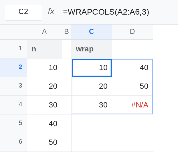
The short last column. In C1 type wrap. Leave C2:D4 empty. In C2 enter =WRAPCOLS(A2:A6,3). Height 3. The spill is C2 10, C3 20, C4 30, D2 40, D3 50, D4 #N/A. Two columns. The last column is short, and the pad fills it. D4 is not a sixth input. Leave D4 as #N/A.

C2 selected. Formula bar shows =WRAPCOLS(A2:A6,3). C2:C4 is 10, 20, 30. D2 is 40, D3 is 50, D4 is #N/A. No other error triangle on C2.

SUM sees the pad. In F1 type total. In F2 enter =SUM(C2:D4). F2 is #N/A. The five numbers are numeric. The sixth cell of the rectangle is not. Leave F2 broken. =SUM(A2:A6) is 150 and never looked at D4.

A chart of the rectangle plots the pad. Select C2:D4. Insert → Chart. Set the chart type to Column chart. In the chart editor, turn off Use row 1 as headers if 10 and 40 were taken as series names instead of values. You get two series (the two columns) and three categories (the three rows of the wrap). The second series has a third point that is #N/A. The column for that point is missing, a gap, not a bar at zero. It is still a slot in the chart. People count three clusters and think a sixth number existed. The source has five numbers. Leave the chart up.

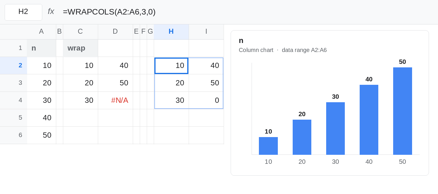
Pad with 0 and the gap becomes a bar. In H2 enter =WRAPCOLS(A2:A6,3,0). The spill is the same shape as C2: H2 10, H3 20, H4 30, I2 40, I3 50, I4 0. The pad is I4, not H4, and it is 0 instead of #N/A. =SUM(H2:I4) is 150, because zero does not break SUM. Select H2:I4 and insert another column chart. The second series now has a bar at zero in the third cluster. That zero is the pad. It is not in A2:A6. Leave I4 as 0 so the fake bar has a cell you can point at.

A label pad is still a category. In H6 enter =WRAPCOLS(A2:A6,3,""). The corner looks blank. A chart of H6:I8 still has three rows of extent if the data range includes the blank. Empty is better than zero for a column chart, and it is worse for a consumer that counts columns. =COUNTA(H6:I8) may still count the five numbers only. =ROWS(H6:I8) is 3 either way. The rectangle did not shrink.

Leave D4 as #N/A and F2 as #N/A. Leave I4 as 0.

What is actually wrong

Output shape is wrap_count rows by enough columns to hold the list. Five items at height 3 is two columns, and 2×3 is six slots. The sixth slot is the pad. D4.
Default pad #N/A poisons SUM, AVERAGE, and any other aggregate that does not ignore errors. F2. It is the same rule as WRAPROWS #N/A pad, on the other axis.
Charts plot the range you give them. The range is the rectangle, pad included. #N/A gaps. 0 draws. See chart error gaps. Neither chart is “wrapping wrong.” C2’s numbers are 10 through 50 in order, down then across.
pad_with "" cleans the corner for the eye and does not remove the row from the spill. ROWS of the block stays 3.
A blocked cell inside the rectangle is #REF! on the formula, which is WRAPCOLS down. D4’s #N/A is a successful wrap. Do not clear a neighbor to fix it.

This is not HSTACK #N/A avg except the same pad idea. HSTACK pads the short array to the tallest. WRAPCOLS pads to a multiple of wrap_count.

Fix

Leave C2’s #N/A and the zero-padded chart in place.

Choose a pad that matches the consumer. If the next step is SUM, do not leave the default. In F4 enter =SUM(WRAPCOLS(A2:A6,3,0)). F4 is 150. If the next step is a column chart, do not use 0. Chart A2:A6, the original list, when the wrap was only for a print layout. If you must chart the wrap, set the chart’s data range to the cells that hold source numbers, or pad with "" and know the blank category is still in a three-row range.

A column chart whose data range is A2:A6, five bars, 10 through 50. Beside it, D4 is still #N/A from WRAPCOLS without pad_with. The pad_with 0 formula is in H2, so H4 is 30 and I4 is 0.

Drop the pad before the chart. =FILTER(TOCOL(C2:D4),ISNUMBER(TOCOL(C2:D4))) returns the five numbers as one column and omits D4. Chart that spill. TOCOL’s ignore argument can drop blanks. #N/A is not a blank. ISNUMBER is the test that fits this pad. See TOCOL / TOROW.

Make the list a multiple of the height only when a genuine sixth value exists. Do not invent 0 in A7 so the wrap comes out even. That zero is the same fake bar, moved into the source.

If the last column is one short and the corner is #N/A, the wrap succeeded. Pass pad_with for SUM. Leave #N/A or chart the source list when a zero would be read as data. If the formula cell is #REF!, the pad is not the problem. Something is sitting in the spill.