Data validation rejects a good number when the custom formula is missing a $

Data → Data validation can use a custom formula. The formula is written for the top-left cell of the validated range, then filled down, the same way conditional formatting fills. A cap that lives in D1 has to be $D$1. Without the dollar signs, row 3 of the range compares itself to D2. D2 is empty. A number that is under the cap is rejected. The dialog says the entry violates the data validation rules. The number was fine. The formula moved.

A dropdown from a range is dropdown range. The same $ idea on a paint rule is conditional formatting $. Keep the Google Sheets UI in English. Sheet Error is an independent formula-error library, not a Google product.

Recreate it on a blank sheet

1. Open a blank spreadsheet. In D1 type 10. That is the cap. In C1 type qty. Leave C2:C5 empty.

The rule. Select C2:C5. Data → Data validation. Add rule. Criteria: Custom formula is. Formula: =C2<=D1. On invalid data, choose Reject the input. Click Done. The range in the rule is C2:C5.

The first cell agrees with you. Click C2 and type 8. It is accepted. 8 is less than or equal to D1, and on C2 the formula really does read D1. Leave 8 in C2.

The next cell rejects the same kind of number. Click C3 and type 8. Sheets rejects it. The message says the data you entered violates the data validation rules set on this cell. 8 does not stay in C3. The cap in D1 is still 10. D2 is blank. On C3 the relative formula became =C3<=D2. A comparison with a blank fails the test you meant. Leave C3 empty. Leave the rule unchanged so the rejection still happens.

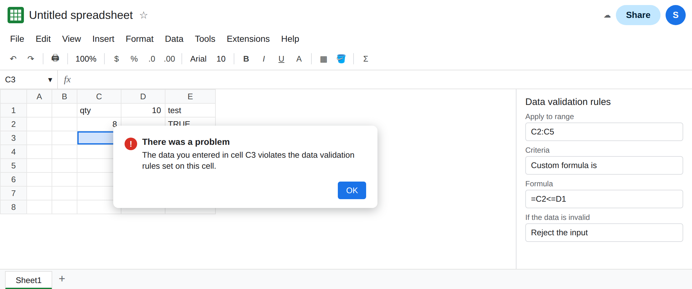
Show a warning would have kept the 8. That choice is the other invalid-data option. It is not this recreate. Reject the input is why C3 is still empty. Do not switch the rule to warning until you have seen the rejection.

A formula you can see. In E2 enter =C2<=D1 and fill E2:E5. E2 is TRUE because C2 is 8 and D1 is 10. E3 is FALSE because C3 is empty and the fill now says =C3<=D2. The validation engine uses that same fill. E3 is not the validation dialog. It is the test, visible. Leave the E column.

This is not a protected cell. A protection dialog names a protected cell or object and does not mention data validation. See protected cell.

What is actually wrong

• One formula is stored for C2. C3, C4, and C5 each get a shifted copy. D1 shifts to D2, D3, and D4 unless you lock it. The cap does not shift. The reference does.
• Reject the input throws the typed value away. You cannot scroll back and find the 8 in C3. The dialog is the only record. A warning would have left the 8 in the cell with a mark. If the 8 is sitting in C3, the rule is not set to reject.
• An empty D2 is not the number 0 for this comparison in the way people hope. The test on row 3 is not “8 <= 10.” Fixing D2 by typing 10 there would make this broken formula pass, and it would hide the missing $. Do not sprinkle the cap down the column to silence the dialog.
• The top-left of the range must be the cell the formula names. If you validate C2:C5 but write =C5<=$D$1, row 2 is tested with a formula that started life aimed at C5. Put C2 in the formula when C2 is the first validated cell.
• Checkbox and dropdown criteria do not use this formula. A list of allowed words rejects 8 because 8 is not in the list. Open the rule and read the criteria before you add dollar signs. See dropdown range.

Conditional formatting will not stop the typed 8. It only paints. A red cell that still holds 8 is a format rule. See CF formula range.

Fix

Leave a copy of the unlocked rule on a second range if you want the rejection to stay reproducible. On C2:C5, lock the cap.

Lock the cell that must not move. Data → Data validation, open the rule, set the formula to =C2<=$D$1. Done. Type 8 in C3. It stays. Type 11 in C4. It is rejected, because 11 is greater than the cap. That rejection is the rule working.

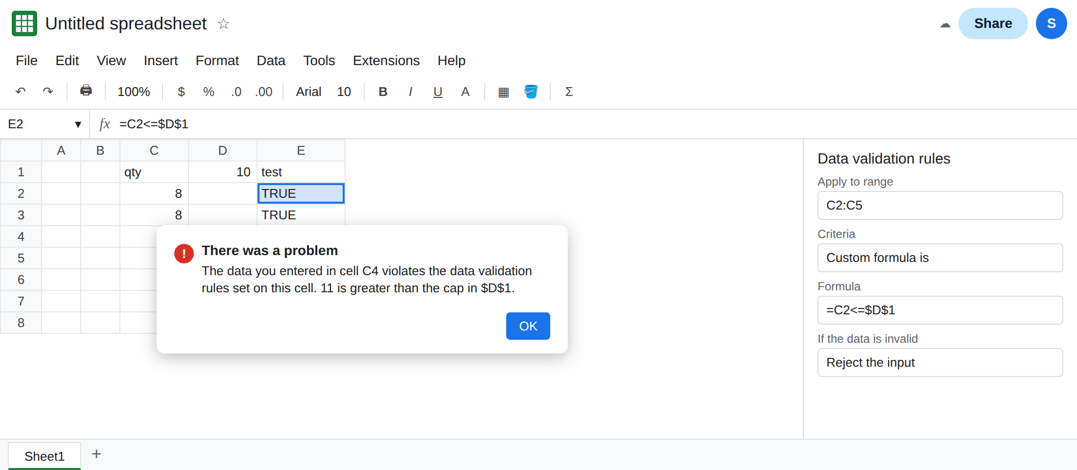
Lock a column when each row has its own limit. A per-row cap in column D uses $D2 so the column stays D and the row follows. $D$1 is wrong for that layout. It would compare every qty to the first cap only.

Do not wrap the validation formula in IFERROR. A formula that errors is an invalid cell, and swallowing the error marks bad input as allowed. Test the formula in column E first. TRUE means accept. FALSE means reject.

If the first cell of the range accepts a number and the cell below rejects the same number, a reference in the formula is relative and the cell it landed on is not the cap. Add $ to the cap. If every cell accepts numbers above the cap, the formula is not the rule that is running. Read the criteria again.