

CLEAN removes ASCII 0–31 and leaves NBSP and zero-width characters
Updated
CLEAN(text) removes the non-printable ASCII characters, codes 0 through 31. That includes tab (CHAR(9)) and the line feed (CHAR(10)). It does not remove the non-breaking space, CHAR(160), and it does not remove the zero-width space, CHAR(8203). TRIM removes ordinary spaces, code 32, and does not remove 160 or 8203 either. After CLEAN, the cell can look like 101 and still fail a lookup. LEN is the check that does not lie.
A SUMIF that skips CHAR(160) is CHAR(160) blanks. This page is CLEAN’s range: what it deletes, and the codes it leaves for that other bug. Keep the Google Sheets UI in English. Sheet Error is an independent formula-error library, not a Google product.
Recreate it on a blank sheet
Section titled “Recreate it on a blank sheet”- Open a blank spreadsheet. In A1 type
raw, B1len, C1clean_len. You will build four dirty codes and one ordinary101.
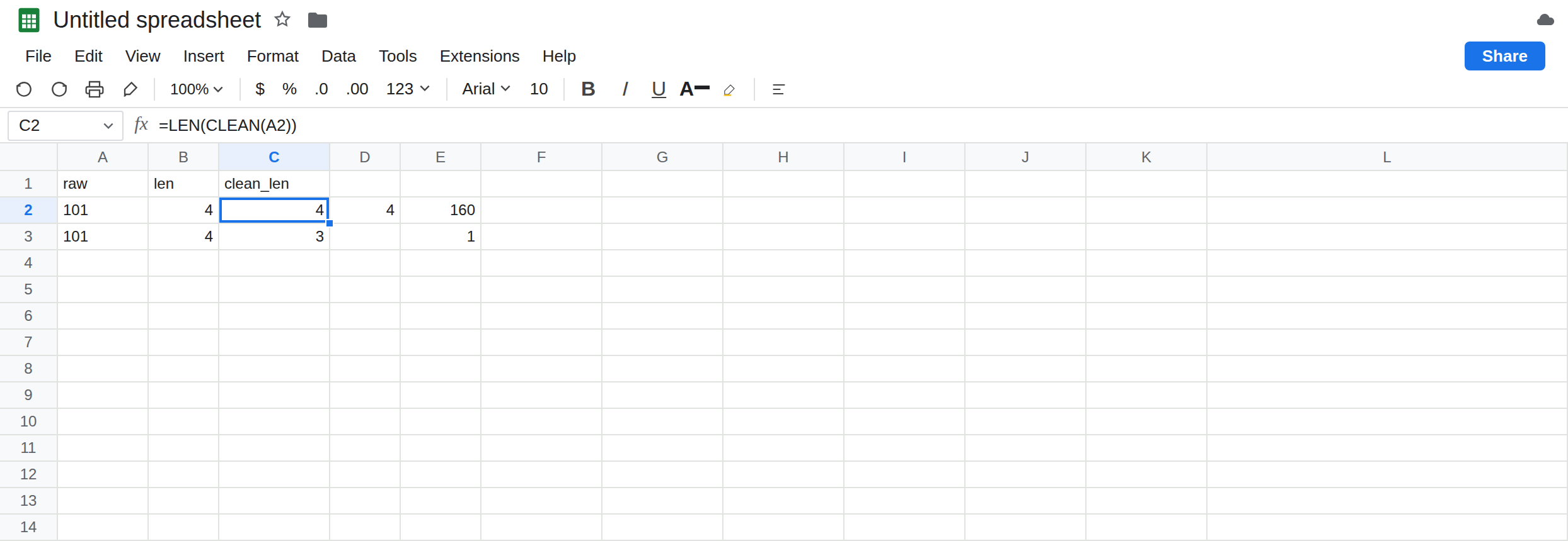
Non-breaking space. In A2 enter ="101"&CHAR(160). The cell looks like 101. In B2 enter =LEN(A2). B2 is 4. In C2 enter =LEN(CLEAN(A2)). C2 is still 4. In D2 enter =LEN(TRIM(A2)). D2 is still 4. In E2 enter =CODE(RIGHT(A2,1)). E2 is 160. CLEAN and TRIM both left the character that CODE can see.
Tab, which CLEAN does remove. In A3 enter ="101"&CHAR(9). B3 =LEN(A3) is 4. C3 =LEN(CLEAN(A3)) is 3. The tab is ASCII 9, inside 0–31. In E3 enter =CODE(RIGHT(CLEAN(A3),1)). E3 is 1, the last digit of 101, because the tab is gone. Leave C2 at 4 and C3 at 3.
Line break. In A4 enter ="N"&CHAR(10)&"12". It may display as two lines. LEN(A4) is 4. LEN(CLEAN(A4)) is 3, and the cleaned text is N12. Line feed is ASCII 10. CLEAN is doing the job it documents. This row is the control.
Zero-width space. In A5 enter ="101"&CHAR(8203). LEN(A5) is 4. LEN(CLEAN(A5)) is 4. LEN(TRIM(A5)) is 4. CODE(RIGHT(A5,1)) is 8203. There is no visible gap. A cursor in the cell still sits past an extra character. Leave this row dirty.
A byte-order mark. In A6 enter ="101"&CHAR(65279). LEN(CLEAN(A6)) is 4. CODE of the last character is 65279. Same story as 8203: not ASCII 0–31, so CLEAN keeps it.
The lookup still misses. In A8 type 101 as a number. In G2 enter =VLOOKUP(101,A2,1,FALSE). The range is only A2, the cell that looks like 101. G2 is #N/A. In G3 enter =VLOOKUP(101,CLEAN(A2),1,FALSE). Still #N/A, because CLEAN did not change A2. Leave G2 and G3 broken. The miss primer for spaces and text-versus-number is VLOOKUP no match. Here the extra character is specifically one CLEAN does not own.
Leave C2 at 4. Leave C3 at 3. Leave G3 as #N/A.
What is actually wrong
Section titled “What is actually wrong”CLEAN’s contract is ASCII non-printables, 0 through 31. Tab and line feed are in that set.CHAR(160)is a space that happens to be outside it.CHAR(8203)andCHAR(65279)are Unicode format characters. The function is not “remove everything I cannot see.”TRIMis ordinary spaces: leading, trailing, and repeated code 32. It does not callCLEAN, andCLEANdoes not callTRIM. A tab might surviveTRIMand die inCLEAN. A non-breaking space survives both. Stacking them withoutSUBSTITUTEstill leaves 160 in the string.LENandCODEare the evidence. IfLENstays 4 afterCLEAN, the extra character is not in 0–31.CODE(RIGHT(...))orCODE(MID(...,n,1))tells you which one.160is the web paste.8203is a rich-text or CMS paste.65279is a file that carried a BOM into the first or last cell.- A lookup of the number
101against text101plus a hidden character is#N/Afor two reasons if you are unlucky: the hidden character, and text versus number. Clean the character first, then compare types. See CSV text vs number if the import itself stored text.CLEANis not an import step. VALUE(CLEAN(A2))is still#VALUE!while the non-breaking space remains. That error is the character, not VALUE() locale.
This is not CHAR(160) blanks as the SUMIF story. Same character, different function. If COUNTIF returns 1, read that page after this one has shown CLEAN will not save the criterion.
This is not a curly quote in a formula. See curly quote parse error. Those break the formula bar. These characters sit in the data.
Leave A2, A5, and G3 dirty.
Strip the codes CLEAN skips, then TRIM and CLEAN. In I2 enter =TRIM(CLEAN(SUBSTITUTE(SUBSTITUTE(A2,CHAR(160)," "),CHAR(8203),""))). I2 is 101. LEN(I2) is 3. The non-breaking space becomes an ordinary space and TRIM can drop it. The zero-width character is deleted, not turned into a space. In I6 enter the same pattern with CHAR(65279) added as another SUBSTITUTE if A6 is in the real column. One SUBSTITUTE per code you found with CODE.
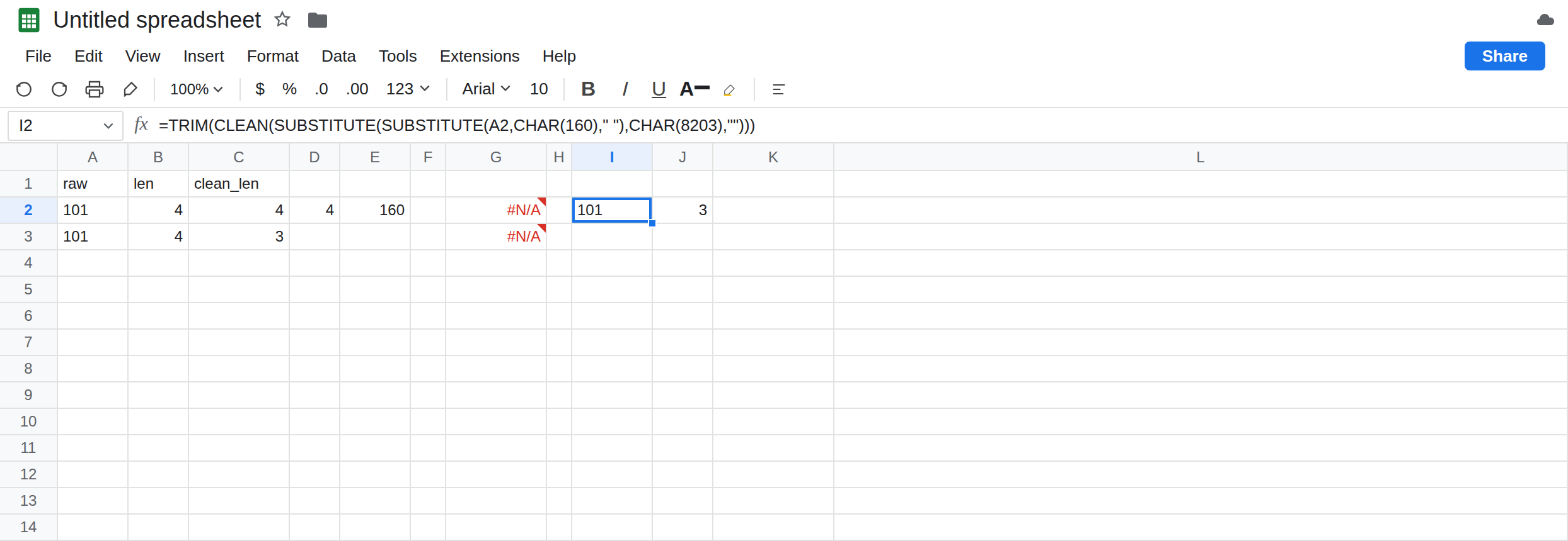
Prove the lookup. In G5 enter =VLOOKUP(101,I2,1,FALSE). If I2 is text 101 and the key is the number 101, Sheets may still match them in VLOOKUP, or you may need VALUE(I2) once LEN is 3. If G5 is #N/A and LEN(I2) is 3, you are on type, not on CLEAN. See VLOOKUP no match.
A tab-only cell. CLEAN(A3) is enough. Do not add three SUBSTITUTE calls because one row had a tab. CODE tells you which row needs which function.
Do not wrap G3 in IFERROR. The #N/A is the character you have not removed. See IFERROR vs IFNA.
If LEN(CLEAN(x)) equals LEN(x) and the cell looks padded or looks fine and still will not match, run CODE on the ends. 160, 8203, and 65279 need SUBSTITUTE. 9 and 10 need CLEAN. 32 needs TRIM.
What CLEAN removes
Section titled “What CLEAN removes”Tab and line feed: length drops. Non-breaking space, zero-width space, and CHAR(65279): length stays, and VLOOKUP of CLEAN is still #N/A. TRIM does not close that gap. SUBSTITUTE of the code you measured, then TRIM and CLEAN, is the string whose length matches the digits you can see.