SUMIF skips text that looks like numbers in the sum range

SUMIF(criteria_range, criterion, sum_range) adds cells in sum_range whose partner row matches. Text in sum_range is not added. A cell that looks like 20 and is actually text adds nothing. The function returns a short total. There is no #VALUE! and no triangle. SUM of that same cell is short for the same reason.

The criteria side is a different coercion. A numeric criterion can still match a text key that looks like that number. Fixing the criterion does not put the text amount into the total.

Recreate it on a blank sheet

1. Open a blank spreadsheet. Keep the Google Sheets UI in English. Confirm File → Settings → Locale is United States so the decimal mark is a period. In A1 type region, B1 amount.

Numbers and one text amount. A2 East, B2 10 typed as a number. A3 East. In B3 type '20 — an apostrophe, then 20 — so the formula bar shows the apostrophe and the cell shows 20 as text. A4 West, B4 30 as a number.

In D1 type east. In D2 enter =SUMIF(A2:A4,"East",B2:B4). The cell shows 10. East has a real 10 and a text 20. Only 10 was added. West’s 30 is a number and is excluded by the criterion, which is correct.

In D4 enter =SUM(B2:B4). The cell shows 40. SUM also skips B3. 10+30 is 40, not 60. The sheet never says B3 is text.

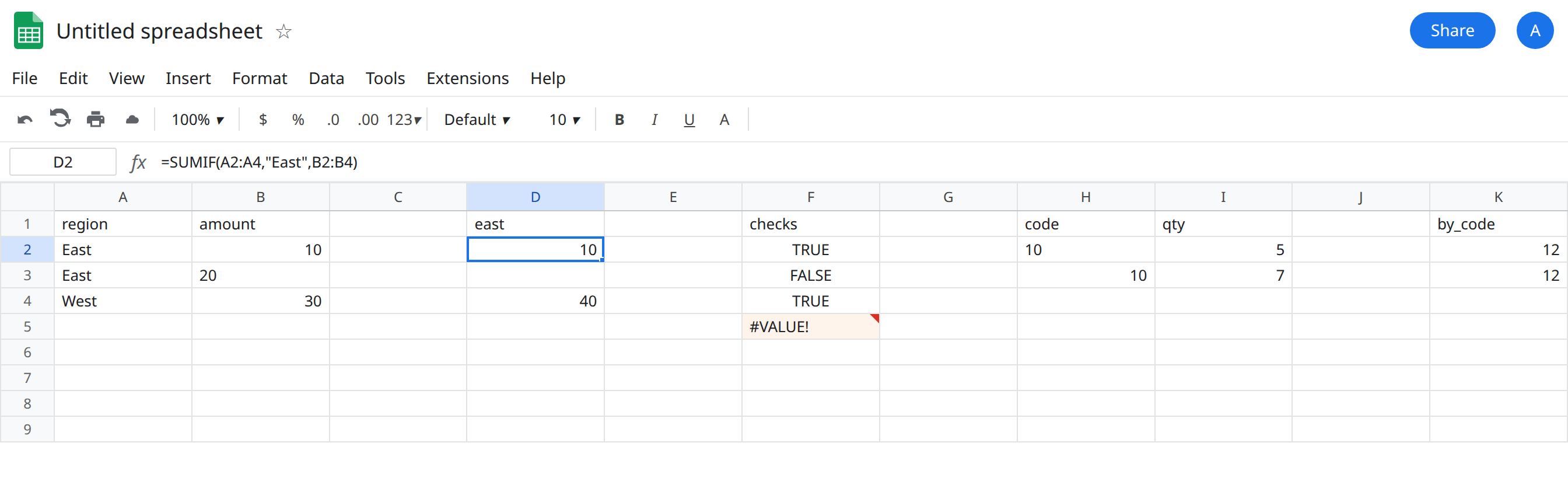
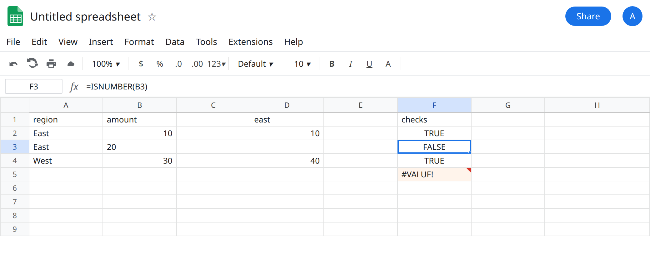
Prove the type. In F1 type checks. F2 =ISNUMBER(B2) TRUE. F3 =ISNUMBER(B3) FALSE. F4 =ISTEXT(B3) TRUE. F5 =B3+0. F5 shows #VALUE!. Arithmetic on the text amount fails. SUMIF does not. It skips. Leave F5 broken so the type error stays visible. Do not “fix” D2 by wrapping it. D2 is not an error.

Criteria that look like numbers, amounts that are real. In H1 type code, I1 qty. H2 type '10 (text). I2 5 as a number. H3 10 as a number. I3 7 as a number. In K1 type by_code. In K2 enter =SUMIF(H2:H3,10,I2:I3). The criterion is a number. In Google Sheets that criterion matches both the text 10 and the numeric 10. K2 shows 12. In K3 enter =SUMIF(H2:H3,"10",I2:I3). K3 is also 12. The criteria matched. The short total on D2 is not this row. D2’s problem is the sum range.

Leave D2 as 10. Leave F5 as #VALUE!.

What is actually wrong

• sum_range is added like SUM. Text, blanks, and booleans do not increment the total. B3 displays 20 because that is what text looks like. ISTEXT is the test that matters. A green triangle or a left alignment is a hint; ISTEXT is the proof.
• Import and CSV files produce this constantly. A column of amounts arrives as text. See CSV text numbers and TO_PURE_NUMBER. SUMIF will not warn you. The region filter still runs.
• The criterion and the sum range follow different rules. K2 shows a numeric criterion matching a text code. People then assume B3 will be added because “Sheets treats 20 as a number.” It treats the criterion loosely. It does not add text.
• A criterion that is itself text with an operator, such as ">10", compares numerically where it can. That does not convert B3 into a number inside the sum.
• Dates stored as text fail a date criterion the same quiet way. See SUMIFS date text. A non-breaking space that makes a code fail to match is CHAR(160) blanks. B3 is not a space. LEN(B3) is 2. The characters are 2 and 0.
• SUMIFS skips text in the sum range too. Extra criteria do not start adding text.

D2 is the dangerous cell because it is a plausible East total if someone forgot the second East row. F5 is the honest cell: #VALUE! means this value is not in the arithmetic.

Fix

Leave D2 and F5 broken.

Convert the sum range, then sum. In B6 enter =TO_PURE_NUMBER(B3). If that returns 20 as a number, the original text can be replaced with values once you trust the column. On a United States locale, =VALUE(B3) is the other converter. See VALUE() locale before you use VALUE on a comma-decimal sheet. After B3 is a real number, D2 becomes 30 without an edit to the formula. The formula was never the bug.

A helper that shows the skip. In D6 enter =SUMPRODUCT((A2:A4="East")*(ISNUMBER(B2:B4))*(B2:B4)). The total is still 10, but you can add a second check: =SUMPRODUCT((A2:A4="East")*(ISTEXT(B2:B4))) is 1. That 1 is the East amount you dropped. Do not replace D2 with IFERROR. There is nothing to catch.

Do not retype the criterion to repair the sum. K3 already matches text keys. Changing "East" to East without quotes is a different bug (#NAME? or a named range), not a path to adding B3.

If SUMIF is smaller than the rows you can see, run ISTEXT down the sum range. The first TRUE on a matching row is an amount that never entered the total.