Fix OFFSET #REF! in Google Sheets when height or width is 0 or negative

OFFSET(reference, rows, cols, [height], [width]) returns a range. Height is how many rows tall that range is. Width is how many columns wide. Both must be greater than 0. 0 is not “use the default.” A negative height is not “count upward,” which is what some Excel files do. Sheets rejects both with #REF!. The starting cell can be legal. The size is what failed.

This page is height and width. It is not OFFSET off sheet (a row or column step that leaves the grid, such as OFFSET(A1,-1,0)). It is not INDEX past range. Keep the Google Sheets UI in English.

Recreate it on a blank sheet

1. Open a blank spreadsheet. In A1 type origin. In A2 type down. In B1 type right. In B2 type far. Four cells. The start of every formula below is A1, which exists.

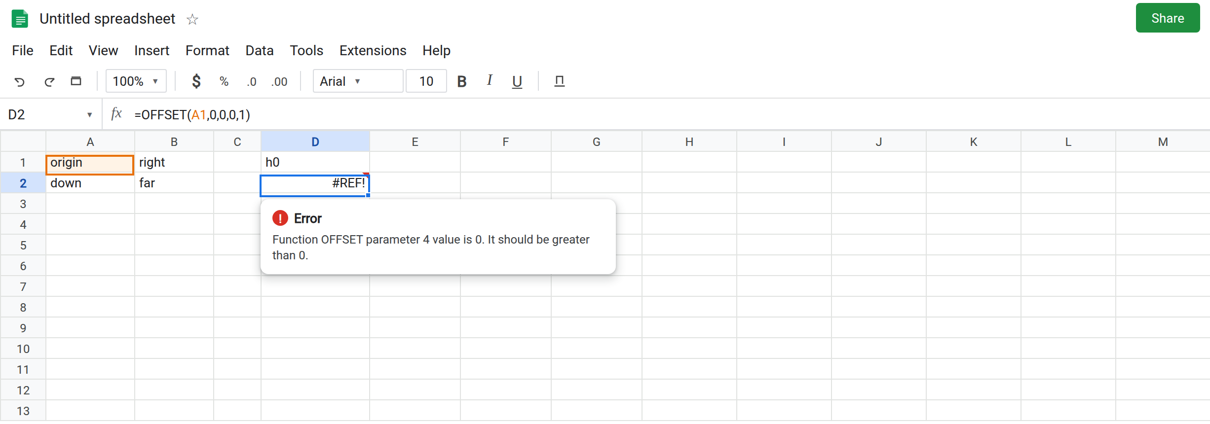
Height 0. In D1 type h0. In D2 enter =OFFSET(A1,0,0,0,1). Rows step 0, columns step 0, height 0, width 1. The anchor is A1. The cell shows #REF!. The tooltip says parameter 4 value is 0 and should be greater than 0. Parameter 4 is height. Leave D2 broken.

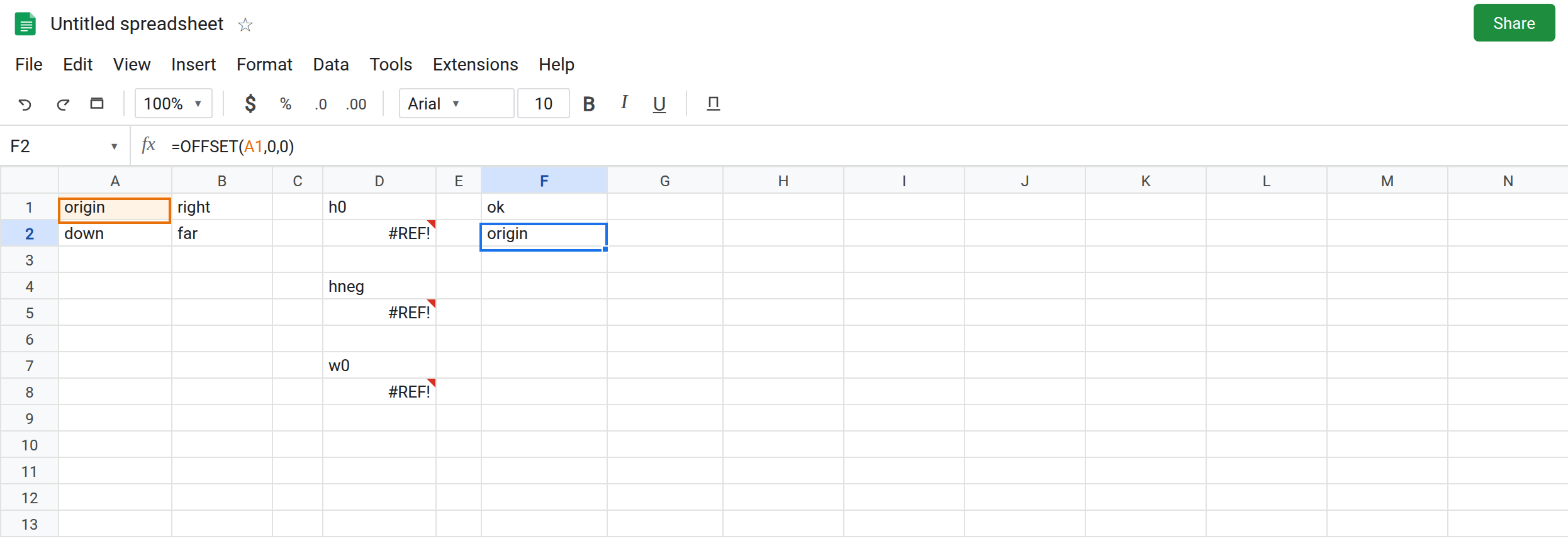
Negative height. In D4 type hneg. In D5 enter =OFFSET(A1,0,0,-2,1). The cell shows #REF!. The tooltip names parameter 4 and the value -2. Sheets did not build a range that grows up from A1. Leave D5 broken. An Excel workbook that used negative height to mean “end above the start” becomes this #REF! on paste.

Width 0. In D7 type w0. In D8 enter =OFFSET(A1,0,0,1,0). Height 1 is legal. Width 0 is parameter 5. #REF!. The tooltip says parameter 5 should be greater than 0. Leave D8 broken.

A one-cell default. In F1 type ok. In F2 enter =OFFSET(A1,0,0). Height and width omitted. The cell shows origin. Omitted means 1 by 1. In F3 enter =OFFSET(A1,0,0,2,2). The formula spills origin / right and down / far if F3:G4 is empty. Height 2, width 2. That block is the control.

A step off the sheet is the other page. In F6 enter =OFFSET(A1,-1,0). Also #REF!, but the bad number is the row step, not height. There is no height argument. That recreate lives on OFFSET off sheet. Leave F6 as the contrast. Do not “fix” it by adding a height.

A blank size from a cell. In H1 type n. Leave H2 empty. In H3 enter =OFFSET(A1,0,0,H2,1). A blank H2 is treated as 0. H3 is #REF!, same as D2. Leave H3 broken. A formula that returns "" into H2 is the same zero.

Leave D2, D5, D8, and H3 broken. Leave F2 as origin.

What is actually wrong

• Height and width are sizes, not directions. Direction is rows and cols, and those may be negative when the landing cell still exists (OFFSET(A2,-1,0) is A1). Size may not be negative.
• Passing 0 because you wanted “default” overrides the default. The default applies only when the argument is absent. D2 passed a zero. F2 passed nothing.
• Parameter numbers in the tooltip: 1 reference, 2 rows, 3 cols, 4 height, 5 width. D8 is parameter 5. Fixing parameter 4 does not clear a zero width.
• A blank driver cell is numeric 0 inside OFFSET. H3. IF(H2="",1,H2) is how you turn “blank means one row” into an explicit 1.
• Negative size is #REF! before any spill. You do not get a range that draws upward and then a second error. The call stops.
• COUNTA or MATCH that returns 0 on an empty list will feed this error the moment it is the height. The tooltip still says OFFSET. The zero was computed upstream.

This is not an index past a named range. See INDEX past range. INDEX does not take a height.

This is not a blocked spill of a legal 2×2. If F3 is #REF! and the tooltip says the array result was not expanded, G3 or F4 is occupied. See SEQUENCE spill for that tooltip family. D2’s tooltip names parameter 4, not a cell to clear.

Fix

Leave D2, D5, and D8 broken.

Use a positive size or omit it. Keep F2 for one cell. For A1:B2 keep a formula with height 2 and width 2 on empty cells: =OFFSET(A1,0,0,2,2).

Blank means 1. In H5 enter =OFFSET(A1,0,0,IF(H2="",1,H2),1). H2 is blank, so the height is 1 and the cell shows origin. When H2 later holds 2, the range becomes two rows. Do not leave the blank to coerce.

Upward in Sheets. Start at the top cell you need and use a positive height. =OFFSET(A1,0,0,2,1) is A1:A2. Do not start at A2 with height -2.

Do not wrap D2 in IFERROR. A zero height would look like an empty origin. See IFERROR vs IFNA.

If the tooltip says parameter 4 or 5 should be greater than 0, the size is the bug. If there is no height argument and the step is negative from row 1 or column A, use the off-sheet page.