

A SPARKLINE stays the default dark line when color or rtl never applied
Updated
SPARKLINE paints one chart in one cell. Color and direction are option pairs, not a second chart type. "color" with a real color string changes the line. "rtl" with the boolean TRUE draws the points from right to left. A misspelled name such as "coulour" does not get ignored. The cell is #N/A, and you never see a black line from that formula. The default dark line is what you get when the formula has numbers and no color pair. People delete the #N/A, leave the color pair out, and describe the dark chart as a typo that Sheets skipped. The typo was an error. The dark line is a different formula.
Illegal charttype values, and the spelling colour, are SPARKLINE charttype. An empty range is SPARKLINE empty / args. Blanks mixed with #N/A are SPARKLINE blanks. Keep the Google Sheets UI in English. Sheet Error is an independent formula-error library, not a Google product.
Recreate it on a blank sheet
Section titled “Recreate it on a blank sheet”- Open a blank spreadsheet. In A1 type
n. A21. A32. A43. A54. A65. The series rises, so a reversed chart is visible.
Default line, no options. In C1 type plain. In C2 enter =SPARKLINE(A2:A6). C2 shows a small line, dark, left to right, low on the left and high on the right. That cell is the control for “default.”
A color that applies. In C4 type blue. In C5 enter =SPARKLINE(A2:A6,{"charttype","line","color","#3366cc"}). C5 shows a blue line of the same numbers. "color" is the option name. #3366cc is a color Sheets accepts. Leave C5 as that blue line.
The typo is an error, not a dark fallback. In C7 type typo. In C8 enter =SPARKLINE(A2:A6,{"charttype","line","coulour","#3366cc"}). The cell shows #N/A. coulour is not an option name. Sheets does not drop the unknown pair and draw C2’s dark line. There is no chart in C8. Leave C8 broken. The spelling colour is the same failure on SPARKLINE charttype.
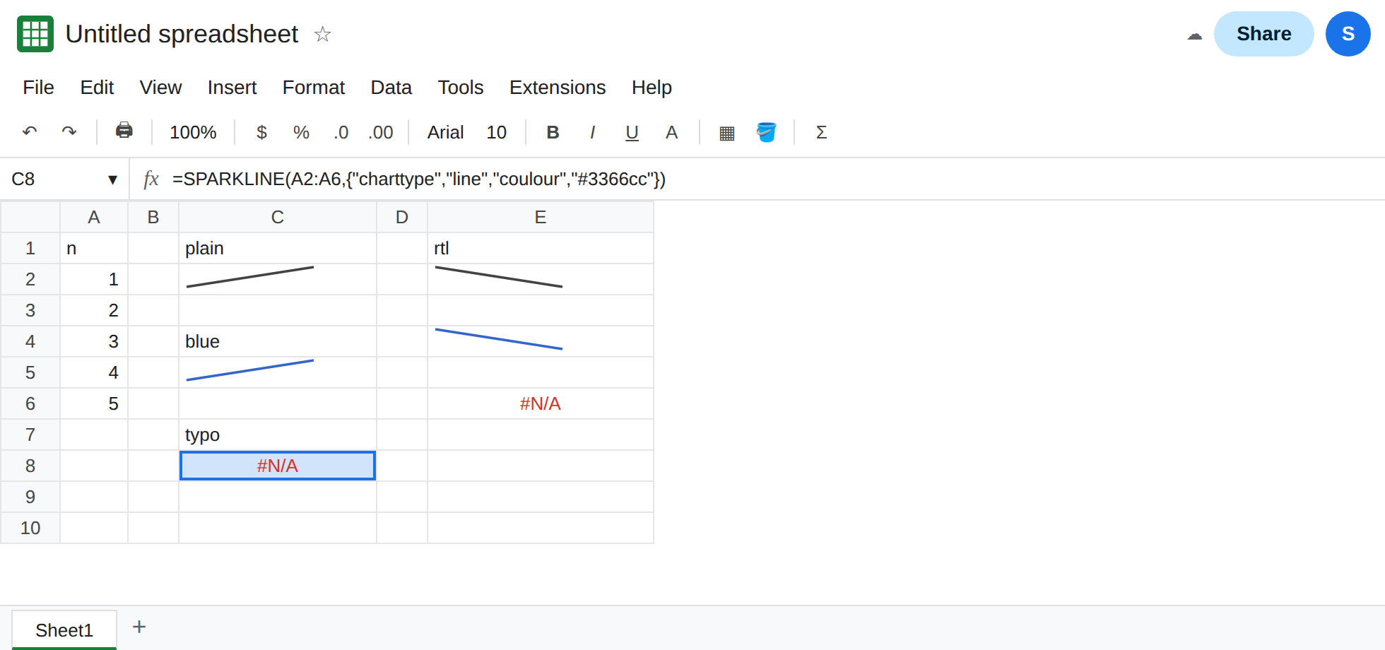
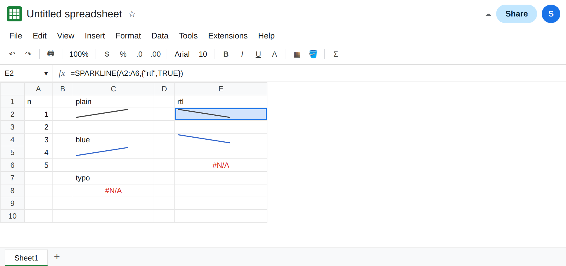
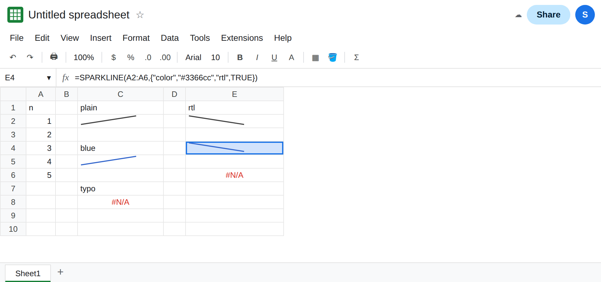
Right to left is a boolean. In E1 type rtl. In E2 enter =SPARKLINE(A2:A6,{"rtl",TRUE}). E2 draws the rise from right to left. The color is still the default dark color. rtl does not set a color. In E4 enter =SPARKLINE(A2:A6,{"color","#3366cc","rtl",TRUE}). E4 is a blue line, reversed. Color and direction are two pairs. In E6 enter =SPARKLINE(A2:A6,{"rtl","yes"}). "yes" is text. E6 is #N/A, or it stays left-to-right if the value is not accepted as true. It is not the E2 reversal. Leave E6 broken if it errors. If it draws left to right, treat it as “the boolean never became TRUE,” and keep E2 as the reversed control.
Bar charts do not use the line’s color key. In E8 enter =SPARKLINE(A2:A6,{"charttype","bar","color","#3366cc"}). The line option "color" is the wrong name for bar. The cell is #N/A, or you do not get the blue you set on C5. Bar colors are "color1" and "color2". In E10 enter =SPARKLINE(A2:A6,{"charttype","bar","color1","#3366cc"}). E10 shows a blue bar chart. Leave E8 as the failed or unchanged attempt. Leave E10 as the bar that took a color.
If { is #ERROR! with Formula parse error, this locale uses \ between array columns. Write {"rtl"\TRUE}. See array literal locale. That parse error is not a color miss.
Leave C8 broken. Leave C2 dark. Leave C5 blue. Leave E2 reversed.
What is actually wrong
Section titled “What is actually wrong”- Option names are exact.
"color"and"rtl"are names."coulour","colour", and"colorr"are not. An unknown name is#N/Afor the whole formula. The chart does not render “except for that pair.” C8 is empty of a chart. C2 is dark because nobody passed"color". "rtl"wants a boolean.TRUEandFALSEare booleans. The word"yes", the word"true", and the number1are not a dependable substitute. E2 is the reversal you can see on 1 through 5. A dark left-to-right line meansrtlis absent or notTRUE. It does not mean the color engine reset itself."color"oncharttypelineis one key."color1"onbaris another. Copying the line’s pair onto a bar is how a bar stays an error, or stays the default, while C5 is blue. Chart types themselves are SPARKLINE charttype.- The options array is pairs. A two-column range on the sheet works the same way as
{name, value}. A typo in the name cell is the same#N/Aas C8.
This is not a sheet chart’s series color. Insert → Chart has its own color controls. See chart error gaps when a line chart skips #N/A. SPARKLINE is a formula.
Leave C8 as #N/A. Leave C2 as the dark line with no options, so the default stays visible.
Spell color, and pass a color. Keep C5: =SPARKLINE(A2:A6,{"charttype","line","color","#3366cc"}). red is also a color. notacolor is not. That bad value is on the charttype page.
Pass TRUE when the series should run right to left. Keep E2. Add the color in the same array when you want both, as in E4. Do not expect "rtl" to change the hue.
For a bar, use color1. Keep E10. Do not keep "color" on a bar and then recolor C5, which is a line.
Do not wrap C8 in IFNA. You would hide an unknown option and show a blank that looks like “no data.” See IFERROR vs IFNA. If the range might be empty, that is the empty-range page, not a color page.
If the line is dark and the formula has no "color" pair, the default is what you asked for. If the cell is #N/A and the option name is coulour, rename it to color. If the line runs left to right, rtl is not the boolean TRUE.