

MATCH type 1 on an unsorted column returns #N/A or the wrong row
Updated
MATCH(key, range, 1) returns the position of the largest value that is less than or equal to the key, and only when the range is sorted ascending. Omit the third argument and Sheets uses 1. On a sku list that was typed out of order, that call is #N/A or a position that is not the exact hit. Exact 0 on the same key still returns the right index. Those are different formulas. A missing sku is a third formula.
This page is approximate MATCH on unsorted data, plus the sorted band where type 1 is intentional. The pure miss — lookup 999, type 0, tooltip Did not find value ‘999’ — is MATCH #N/A. That page also records type 1 on 101, 103, 102 looking up 102 as #N/A. Do not rebuild that grid here and invent a different index for it.
Recreate it on a blank sheet
Section titled “Recreate it on a blank sheet”- Open a blank spreadsheet. You are building quantity breaks, not skus. Keep the Google Sheets UI in English.
Sorted band (the control). In A1 type min_qty. A2 0. A3 100. A4 500. The list ascends. In C1 type lookup. C2 250. C3 100.
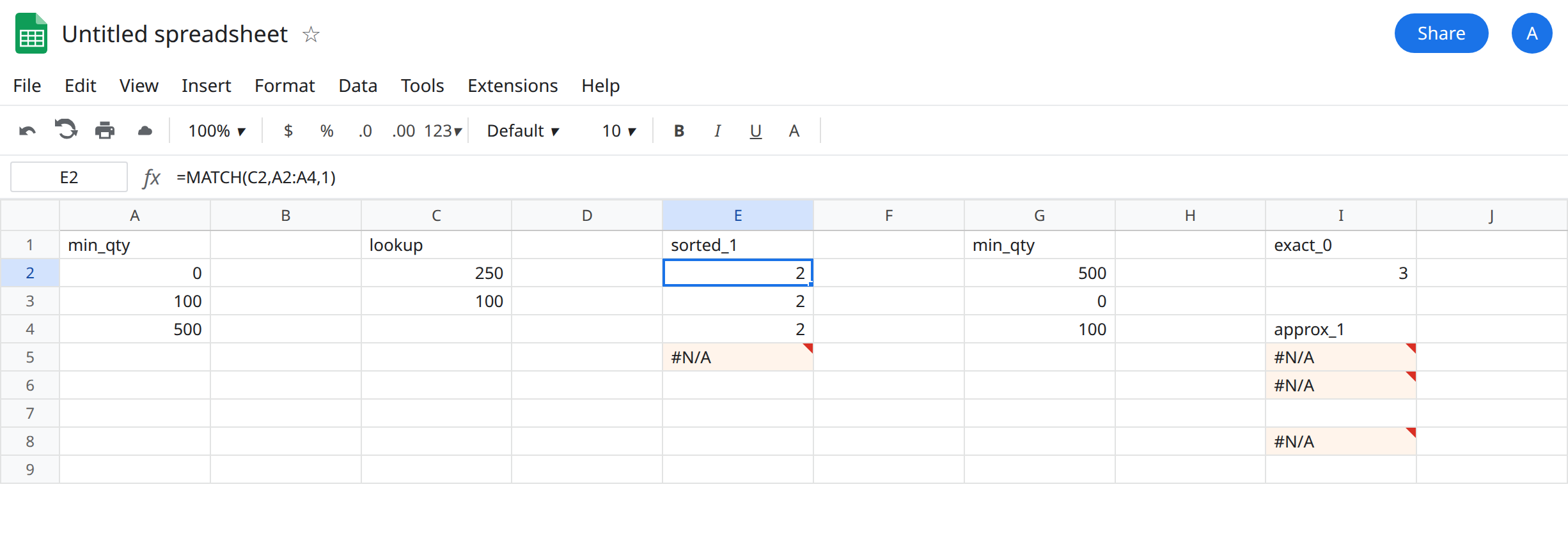
In E1 type sorted_1. In E2 enter =MATCH(C2,A2:A4,1). The cell shows 2. Break 100 is the largest minimum that is still <= 250. Position 2 is correct approximate behavior. In E3 enter =MATCH(C3,A2:A4,1). The cell shows 2. In E4 enter =MATCH(C3,A2:A4,0). The cell shows 2. On a sorted list, an exact key agrees with type 1 and type 0.
Exact miss of a qty that is not a break. In E5 enter =MATCH(C2,A2:A4,0). The cell shows #N/A. The tooltip is Did not find value ‘250’ in MATCH evaluation. 250 is not a listed minimum. Type 0 is supposed to fail. That #N/A is not the unsorted bug. Leave E5 broken.
Same keys, not sorted. In G1 type min_qty. G2 500. G3 0. G4 100. In I1 type exact_0. In I2 enter =MATCH(C3,G2:G4,0). The cell shows 3. Value 100 is the third cell. Exact match does not care about order.
Type 1 on that unsorted column. In I4 type approx_1. In I5 enter =MATCH(C3,G2:G4,1). I5 is #N/A or some position that is not 3. It is not the exact hit you just proved in I2. In I6 enter =MATCH(C3,G2:G4) with no third argument. I6 matches I5. Omitted means 1. Leave both if they are not 3.
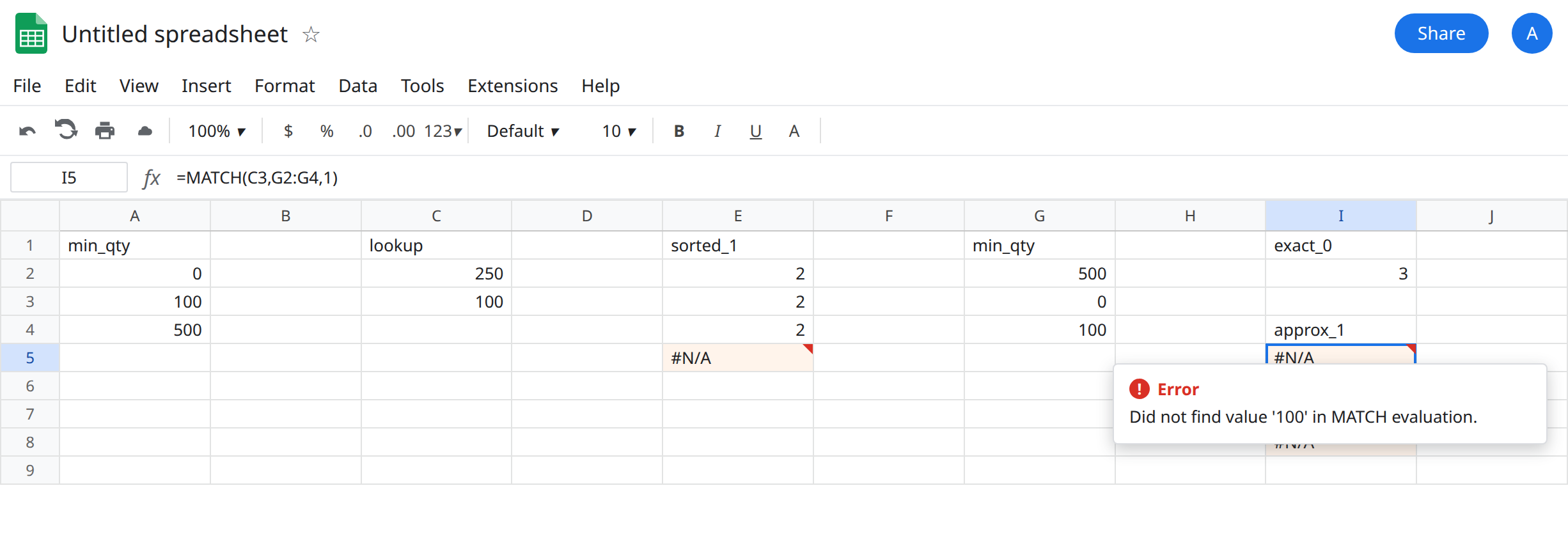
In-between key on the unsorted column. In I8 enter =MATCH(C2,G2:G4,1). 250’s correct band on the sorted sheet was position 2 (the cell holding 100). On G2:G4 the cell holding 100 is position 3. I8 is #N/A or a position that is not that band. Do not write a guessed index into the sheet. Sheets does not promise one stable wrong row for every unsorted list. Compare I8 with E2.
Leave I5, I6, I8, and E5 broken. Leave E2 as 2 and I2 as 3.
What is actually wrong
Section titled “What is actually wrong”match_type1is approximate, ascending. The contract is “largest value<=key.” That contract is true for A2:A4. It is not true for G2:G4. G2 starts at500, then drops to0.- The third argument defaults to
1. A formula copied from a bracket example onto a sku column silently becomes approximate. I6 proves the default: it copies I5, not I2. - Unsorted approximate results are not a single published index. On this grid, type
1of100is not3. It may be#N/A(tooltip Did not find value ‘100’ in MATCH evaluation) or another position. The MATCH #N/A recreate used101,103,102and recorded#N/Afor type1of102. A different unsorted list can land on a wrong index instead. Both outcomes mean “do not use type1here.” Neither outcome means the key is absent: I2 already found100. - Type
0of250on the sorted breaks is#N/Aon purpose.250is between breaks. People “fix” E5 by switching to type1without sorting, then trust I8. E2 is the sorted answer. I8 is not a shortcut to E2. - Type
-1wants descending order. It is the same class of bug on G2:G4. This page stays on type1because that is the default.
This is not an exact miss of 999. See MATCH #N/A. This is not VLOOKUP returning a name. Approximate VLOOKUP is VLOOKUP TRUE bands and the sku version is VLOOKUP wrong row. MATCH returns a position. You still need INDEX if you want the price.
XLOOKUP neighbor modes are a different argument list. See XLOOKUP match_mode.
Leave I5, I6, I8, and E5 on the sheet.
Sku or any key that must be exact. Use type 0. I2 is already =MATCH(C3,G2:G4,0). For a missing key that should print a label, wrap only that form: =IFNA(MATCH(C2,G2:G4,0),"none"). Use IFNA, not IFERROR. See IFERROR vs IFNA. Do not wrap I5. An approximate #N/A on an unsorted list is a match_type bug. Hiding it reports “none” for a key that I2 can see.
Quantity breaks: sort, then type 1. Keep E2: =MATCH(C2,A2:A4,1) is 2. If you insert a row, sort A2:A before you trust type 1 again. Do not sort a sku column to make the default look right.
Read the position with INDEX only after the position is the one you meant. =INDEX(B2:B4,E2) belongs on the sorted breaks. Pointing INDEX at I5 publishes the wrong row with no new error.
If MATCH of a key you can see with type 0 is a different index or #N/A under type 1, the column is not an ascending band. Pass 0, or sort and keep 1 on purpose.