Fix SORT #N/A in Google Sheets (sort column height does not match)

SORT(range, sort_column, is_ascending) can sort by a column outside range. That outside column must be a single column with the same number of rows as range. Three data rows and two key rows is #N/A. The tooltip is SORT has mismatched range sizes. The rows never move. A blocked spill is a different #REF! and only happens after the heights already match.

Google Sheets has no SORTBY. A pasted =SORTBY(...) is #NAME? (unknown function). This page does not use that name. The height rule is SORT.

This page is the outside key’s height. It is not SORT / UNIQUE spill (the list sorts, then a cell in the way is #REF!). It is not SORTN n / ties. Keep the Google Sheets UI in English.

Recreate it on a blank sheet

1. Open a blank spreadsheet. In A1 type sku, B1 name, C1 priority. A2 101, B2 Widget, C2 2. A3 102, B3 Gadget, C3 1. A4 103, B4 Lamp, C4 3. Three data rows. Priority is the sort key, and it is not inside A:B.

Key shorter than the data. In E1 type short_key. In E2 enter =SORT(A2:B4,C2:C3,TRUE). A2:B4 is three rows. C2:C3 is two. The cell shows #N/A. The tooltip is SORT has mismatched range sizes. Expected row count: 3. column count: 1. Actual row count: 2, column count: 1. Priority 3 in C4 was left out, so the rows cannot pair. Leave E2 broken.

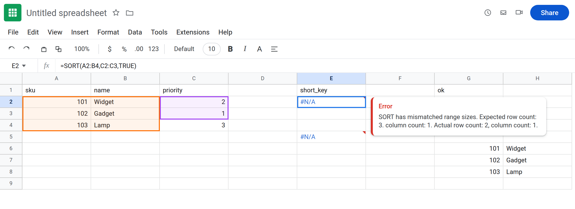
Key wider than one column. In E5 enter =SORT(A2:B4,C2:D4,TRUE). sort_column must be one column. C2:D4 is two wide. #N/A, mismatched range sizes, column count 2 rather than 1. Leave E5 broken.

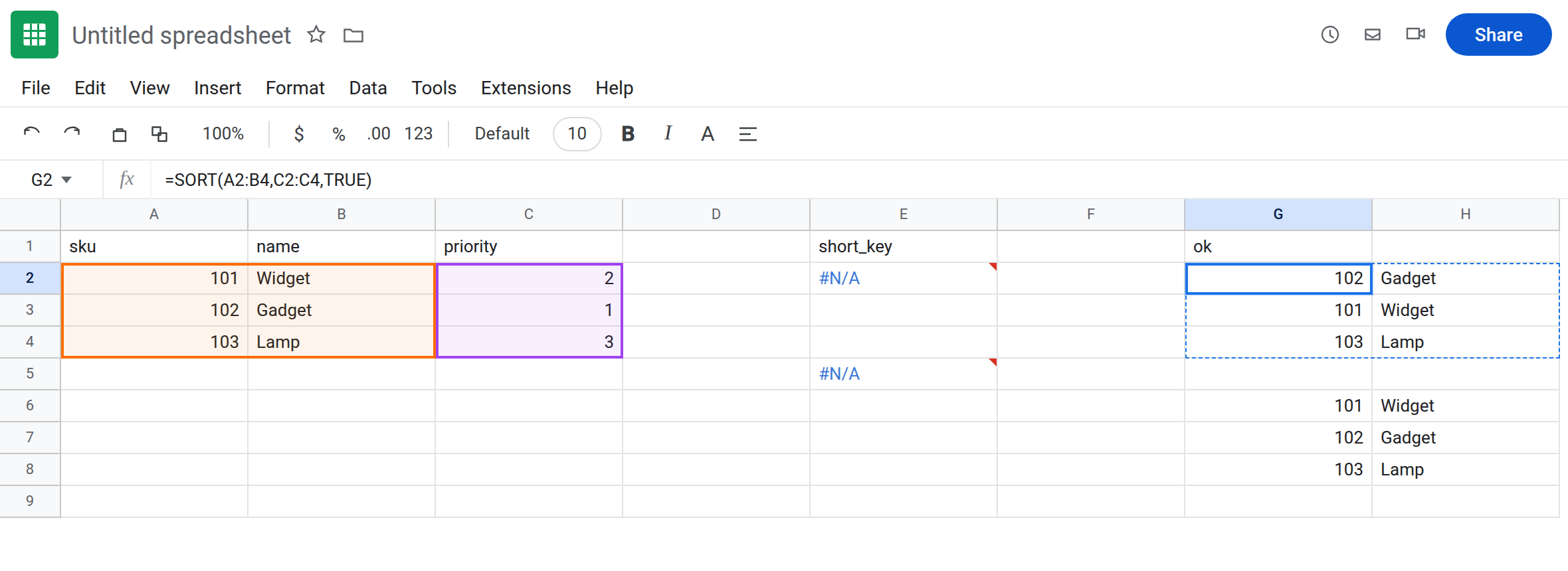
A key that matches. In G1 type ok. Leave G2:H4 empty. In G2 enter =SORT(A2:B4,C2:C4,TRUE). The spill is 102 / Gadget, then 101 / Widget, then 103 / Lamp. Columns stay sku, name. Priorities 1, 2, 3 decide the order and are not copied into the spill. That block is the control.

Inside-column index, for contrast. In G6 enter =SORT(A2:B4,1,TRUE). Sort column 1 means the first column of A2:B4 (sku). The spill is 101, 102, 103. Heights are not in question. The order is sku order, not priority. If you wanted priority and you see 101 first, you passed an index instead of C2:C4. No error triangle. Leave G6 as that contrast.

Spill is a different error. G2 is clear, so it spills. If a later edit puts a value in H3, G2 becomes #REF! and the tooltip is Array result was not expanded because it would overwrite data in ‘H3’. The key was already height 3. That page is SORT / UNIQUE spill. Undo the value so G2 stays the control. Do not lengthen C2:C3 to fix a tooltip that names a cell.

Leave E2 and E5 as #N/A. Leave G2 as the priority order.

What is actually wrong

• An outside sort_column is zipped to range by row. Row 1 of the data with row 1 of the key. Three and two cannot zip. The tooltip’s expected row count is the data. The actual row count is the key. E2.
• The key is one column. A two-column “priority and sku” block is not one sort_column. A second key is another pair: =SORT(A2:B4,C2:C4,TRUE,A2:A4,TRUE) — priority, then sku. Each outside range must still be height 3.
• TRUE is ascending, FALSE is descending. E2 already passes TRUE. The flag is not why the tooltip counts rows. Omitting is_ascending is a different argument error (SORT expects the column and the flag in pairs).
• FILTER then SORT breaks the same way when the key is the unfiltered column. =SORT(FILTER(A2:B4,C2:C4=1),C2:C4,TRUE) filters the data down to the rows with priority 1, then sorts those rows by all of C2:C4. The filtered array is shorter than three. #N/A, mismatched sizes. Filter the key with the same condition, or include priority inside the filtered range and sort by its index.
• Excel’s SORTBY is not on the English Sheets function list. =SORTBY(A2:B4,C2:C4) is #NAME?, Unknown function: ‘SORTBY’. See unknown function. Rewriting that call into SORT is how you reach this page’s height rule. This page’s broken cell is E2, and E2 says SORT.

This is not a blocked spill. See SORT / UNIQUE spill. E2’s tooltip does not name a cell that would be overwritten. The formula did not get far enough to spill.

This is not FILTER’s own size error. See FILTER range size. If the tooltip says SORT, you are here. If it says FILTER, the condition height is wrong before any sort.

This is not SORTN with n of 0. See SORTN n / ties. SORTN can take an outside column too, and that column has the same height rule, but E2 is SORT.

Fix

Leave E2 and E5 broken.

Make the key the same height, one column wide. Keep G2: =SORT(A2:B4,C2:C4,TRUE). If rows are filtered, filter both sides:

=SORT(FILTER(A2:B4,C2:C4>=1),FILTER(C2:C4,C2:C4>=1),TRUE)

On this sheet every priority is at least 1, so that matches G2’s order. The two FILTER results have the same row count. Sorting the filtered block by column index 1 instead is sku order again — only do that if sku is the key you wanted.

Do not wrap E2 in IFNA. A short key is not a missing sku. See IFERROR vs IFNA. You would hide the height bug and show a blank.

If SORT is #N/A and the tooltip says mismatched range sizes, count key rows against data rows, and count key columns (must be 1). If SORT is #REF! and the tooltip names a cell, the heights match — clear the spill. If the formula bar says SORTBY, that function is not in Sheets.