Fix ARRAYFORMULA with AND/OR in Google Sheets (one TRUE/FALSE for the whole column)

AND and OR always return one boolean. Wrapped in ARRAYFORMULA, they still collapse the whole range. AND(A2:A4="East", B2:B4>10) is FALSE if any row fails, even when row 2 is East and over 10. The grid looks like every condition is wrong. There is often no red triangle on that single FALSE. FILTER then sees a one-cell condition against three data rows and reports mismatched range sizes — not “no matches” for a missing sku.

This page is AND / OR inside an array. It is not ARRAYFORMULA empty 0 (blank × 2 prints 0). It is not FILTER no match (A2:A4=999). Keep the Google Sheets UI in English.

Recreate it on a blank sheet

1. Open a blank spreadsheet. In A1 type region, B1 qty. A2 East, B2 12. A3 West, B3 20. A4 East, B4 4. Only row 2 is East and quantity over 10. Row 4 is East but the quantity is 4. Row 3 is over 10 but West.

AND collapses. In D1 type and_all. In D2 enter =ARRAYFORMULA(AND(A2:A4="East",B2:B4>10)). The cell shows FALSE. One cell. Not a spill of TRUE / FALSE / FALSE. Row 2 met both tests, and the formula still says FALSE, because AND required every pair in the two ranges. Leave D2 as FALSE.

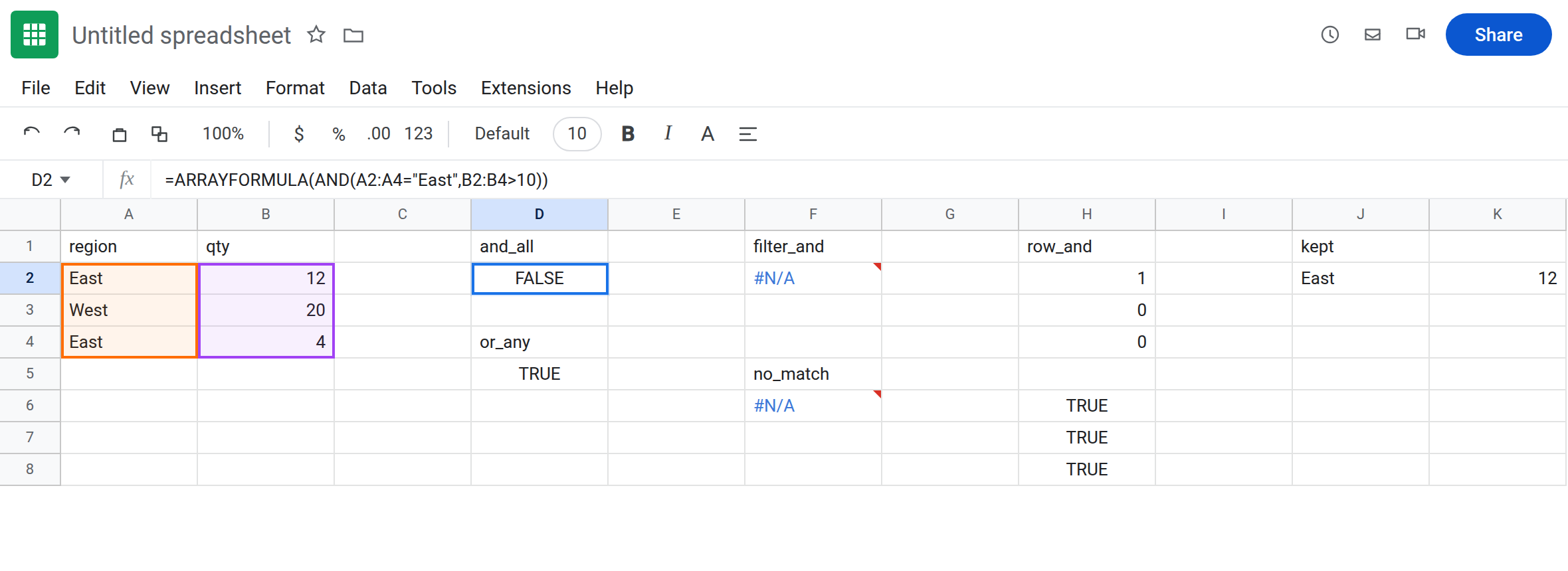
OR collapses the other way. In D4 type or_any. In D5 enter =ARRAYFORMULA(OR(A2:A4="East",B2:B4>10)). The cell shows TRUE. One cell. West with 20 made the whole OR true, and East with 4 did too. You cannot see which row qualified. Leave D5 as TRUE.

FILTER inherits the one-cell condition. In F1 type filter_and. In F2 enter =FILTER(A2:B4,AND(A2:A4="East",B2:B4>10)). The cell shows #N/A. The tooltip is FILTER has mismatched range sizes. Expected row count: 3. column count: 1. Actual row count: 1, column count: 1. AND already reduced the condition to one boolean. FILTER will not broadcast that boolean down the three rows. Leave F2 broken.

Per-row AND that works. In H1 type row_and. Leave H2:H4 empty. In H2 enter =ARRAYFORMULA((A2:A4="East")*(B2:B4>10)). The column spills 1, 0, 0. 1 is row 2 only. That block is the control.

Per-row OR. In H6 enter =ARRAYFORMULA(((A2:A4="East")+(B2:B4>10))>0). The column spills TRUE, TRUE, TRUE. East qualifies, and West qualifies because 20 is over 10. A row that is West with quantity 3 would be FALSE. On this sheet every row has one of the two flags.

Zero-row contrast. In F6 enter =FILTER(A2:B4,A2:A4=999). #N/A, tooltip No matches are found in FILTER evaluation. Same error value as F2, different tooltip. That page is FILTER no match. Leave F6 as contrast.

Leave D2, D5, and F2 as the collapsed results. Leave H2 as 1, 0, 0.

What is actually wrong

• AND is true only when every argument is true. Passed two ranges, it looks at the whole blocks, then returns one boolean. ARRAYFORMULA does not turn AND into a row-by-row function. D2 is that single FALSE.
• OR is true when any argument is true. D5 is one TRUE for the entire list. A later IF(D5,"keep","drop") would keep or drop all rows together.
• Multiplication is the array form of AND: TRUE is 1, FALSE is 0, and 1*0 is 0. Addition is the array form of OR. >0 turns 1 or 2 back into a boolean so a row that matches both flags is still just TRUE.
• FILTER wants the condition to have the same height as the data. A one-cell AND is height 1. The tooltip counts rows. It does not say the region is missing. F2 is FILTER range size caused by AND, not by a range you typed too tall.
• IFS and IF have the same habit if you wrap AND of whole columns inside them. The per-row tests belong in the multiplication, and IF can sit outside: =ARRAYFORMULA(IF((A2:A4="East")*(B2:B4>10),B2:B4,"")).

This is not blank cells becoming 0 under A2:A4*2. See ARRAYFORMULA empty 0. H2’s zeros are failed conditions, not empty quantities coerced to zero.

This is not FILTER of sku 999. See FILTER no match. Read the tooltip. Mismatched range sizes means the condition shrank. No matches means the condition was the right shape and nothing was TRUE.

Fix

Leave D2, D5, and F2 broken.

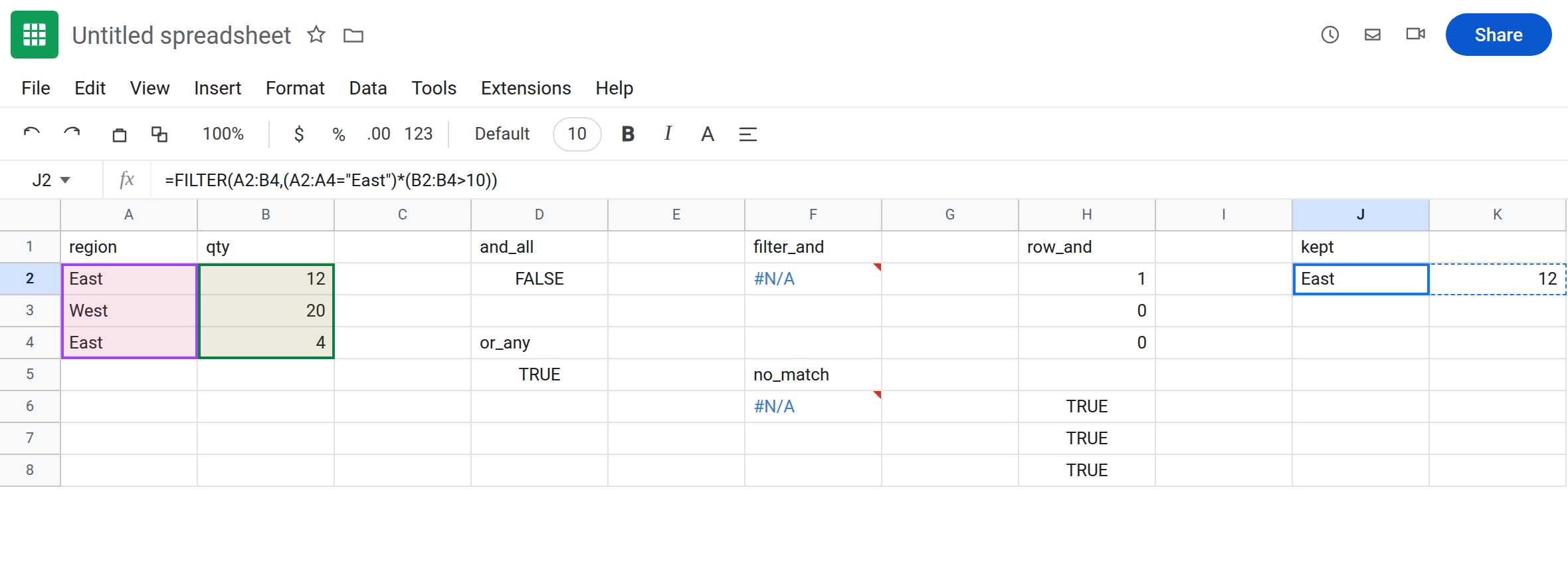
Multiply for AND, add for OR. Keep H2. In J1 type kept. Leave J2:K2 empty. In J2 enter =FILTER(A2:B4,(A2:A4="East")*(B2:B4>10)). The spill is East / 12 only. No AND call.

OR in FILTER. =FILTER(A2:B4,(A2:A4="East")+(B2:B4>10)). A sum of 1 or 2 is truthy. You do not need >0 inside FILTER. You do need >0 if the next function must see TRUE/FALSE rather than 2.

When the test is too awkward to multiply, run AND on one row at a time: =BYROW(A2:B4,LAMBDA(r,AND(INDEX(r,1)="East",INDEX(r,2)>10))). Each call gets scalars, so AND is legal. If that lambda returns an array, you are on BYROW / MAP LAMBDA. Do not put AND back around the whole columns to “simplify” it.

Do not wrap D2 in IFERROR. FALSE is not an error. Do not switch locale. The formula parsed.

If ARRAYFORMULA of AND or OR is a single boolean, the function aggregated the range. Rebuild the mask with * and +. If FILTER then says actual row count 1, you passed that single boolean in as the condition.