

Fix DATEVALUE #VALUE! in Google Sheets (text the locale will not parse)
Updated
DATEVALUE turns a date written as text into a Sheets date serial. #VALUE! means that string is not a date this spreadsheet’s locale will parse. The function name is fine. The text is the wrong shape for this file’s date convention, or it is not a date at all.
This page is locale-shaped date text. It is not wrong type as a generic primer (10 + pcs, DATEVALUE("Widget") as a non-date word). It is not QUERY mixed dates (year(A) on a column that mixes dates with TBD). Keep the Google Sheets UI in English. Locale is File → Settings → Locale, not the display language.
Recreate it on a blank sheet
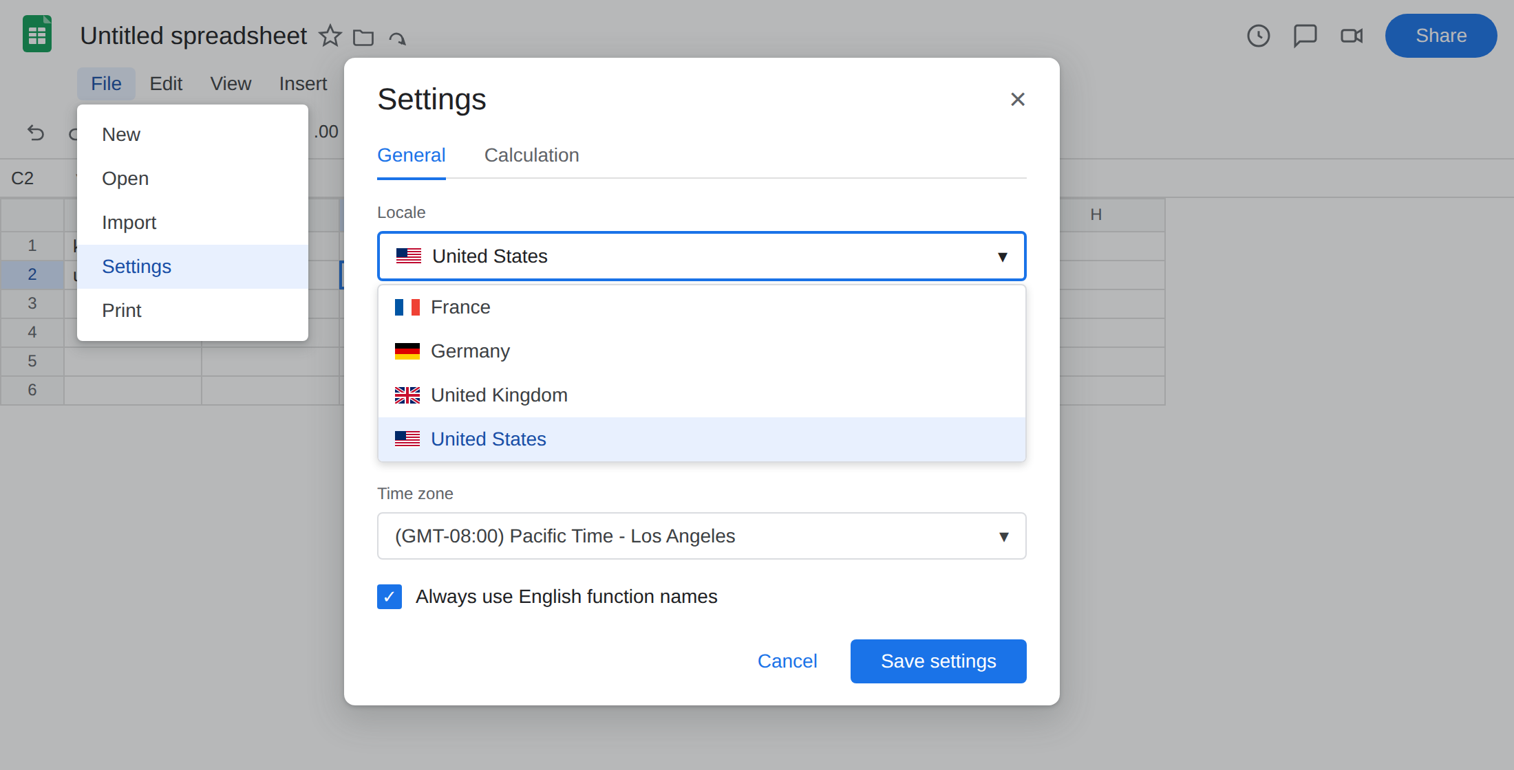
Section titled “Recreate it on a blank sheet”- Open a blank spreadsheet. File → Settings. Set Display language to English if it is not already. Set Locale to United States. Save. United States reads dates as
M/D/Y. - In A1 type
kind, B1text, C1datevalue. - A US string this locale accepts. In A2 type
us_ok. In B2 type1/13/2024as text (type an apostrophe then1/13/2024so Sheets does not auto-convert to a date). In C2 enter=DATEVALUE(B2). The cell shows a date (January 13, 2024). Format C2 as a date if you only see a serial. That row is the control:DATEVALUEworks when the string matches the locale.
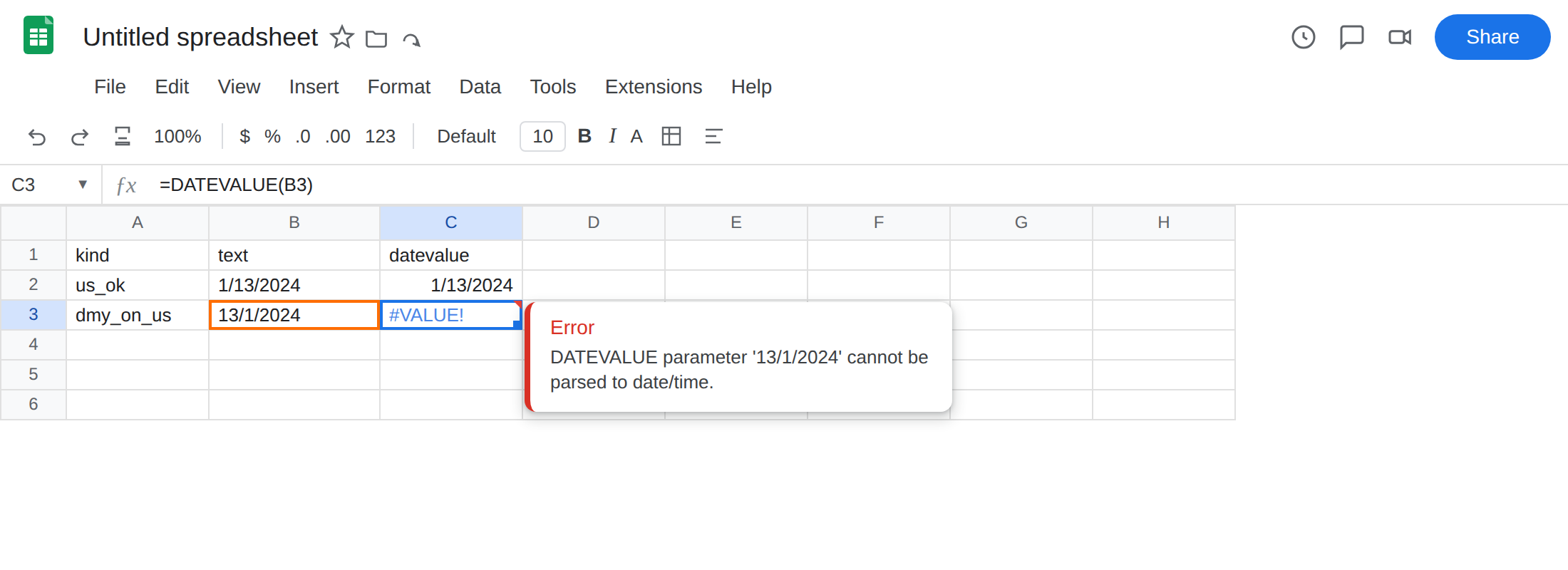
- A D/M/Y string this US locale will not parse. In A3 type
dmy_on_us. In B3 type an apostrophe then13/1/2024(day 13, month 1). In C3 enter=DATEVALUE(B3). The cell shows#VALUE!. United States treats the first number as the month. There is no month 13. Leave C3 broken.
- The reverse locale. File → Settings → Locale → United Kingdom (English UI stays English). United Kingdom reads
D/M/Y. C3 may become a date (13 January 2024). C2 may become#VALUE!because1/13/2024is now day 1, month 13 — and there is no month 13. That toggle is the point: the same strings swap who fails. Set Locale back to United States so the rest of this page matches the broken C3 you started with, or leave UK and treat C2 as the broken cell. Do not change Display language.
ISO-shaped text. In A5 type iso. In B5 type '2024-01-13. In C5 enter =DATEVALUE(B5). This often succeeds on both locales because yyyy-mm-dd is unambiguous. If C5 is a date while C3 is #VALUE!, the failure is the M/D/Y vs D/M/Y string, not DATEVALUE as a whole.
Leave the broken locale string as #VALUE!. Leave the matching-locale string as the working control.
What is actually wrong
Section titled “What is actually wrong”DATEVALUEparses text with this spreadsheet’s locale. United States:1/13/2024is January 13.13/1/2024is month 13.#VALUE!. United Kingdom: the same pair flips.- Auto-conversion hides the bug. If you type
1/13/2024without an apostrophe on a US sheet, Sheets may store a real date beforeDATEVALUEruns. The recreate uses a leading apostrophe so the cell stays text.ISTEXT(B3)should be TRUE.ISNUMBER(B3)should be FALSE. - A word is a different
#VALUE!.=DATEVALUE("Widget")fails on every locale. That is wrong type. This page is a string that is a date somewhere, and not here. DATEVALUEof a cell that is already a date serial can still work (Sheets will coerce), but that is not this recreate. The failure is unparsable text.- Changing the formula to
VALUEdoes not pick a date convention for you.VALUE("13/1/2024")on a US locale is the same class of refusal.
This is not QUERY year(A) on dates mixed with TBD. QUERY types a column. One text TBD makes year(A) #VALUE! with Can’t perform the function year on a column that is not a Date or a DateTime column. See QUERY mixed dates. C3 is a single DATEVALUE call. There is no TBD in the column.
This is not a Formula parse error from commas vs semicolons. See locale parse error. C3 parsed. Then DATEVALUE rejected the string.
This is not #N/A. Nothing is being looked up. See what #N/A means.
Leave the mismatched-locale cell broken so #VALUE! stays on the sheet.
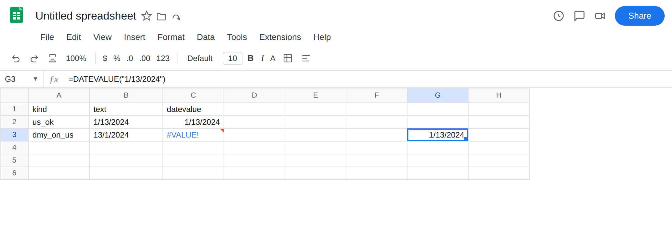
Write the date in this locale’s order. On United States, keep B2 (1/13/2024) and C2. For a 13 January date as text, type '1/13/2024 or 'January 13, 2024, not '13/1/2024. In G3 enter =DATEVALUE("1/13/2024"). The cell matches C2.
Prefer an unambiguous string. =DATEVALUE("2024-01-13") (ISO) or =DATE(2024,1,13) (numbers, no locale order). DATE does not parse text. Year, month, day are already numbers. Use DATE when the parts live in separate cells.
Do not “fix” a UK sheet by pasting US strings. If the file’s locale is United Kingdom on purpose, write 13/1/2024 or ISO. Do not set Locale to United States to make one formula work and break every dd/mm date already on the file.
Convert a real date, not DATEVALUE of a date. If B2 already became a date (no apostrophe), you do not need DATEVALUE. Use the cell. DATEVALUE is for leftover text from CSV, concat, or another system.
Do not wrap this #VALUE! in IFERROR and call the date fixed. You still do not have January 13. Match the string to File → Settings → Locale, or stop parsing text and pass DATE(year, month, day).