

Fix ARRAYFORMULA 0 on empty rows in Google Sheets
Updated
An empty qty row still shows 0 after ARRAYFORMULA multiplies the column. That is not a formula error. Sheets treated the blank as 0. The formula ran. There is no red triangle. A later COUNT or SUM will treat that 0 as a real value unless you stop writing it.
Recreate it on a blank sheet
Section titled “Recreate it on a blank sheet”- Open a blank spreadsheet. Leave the tab named
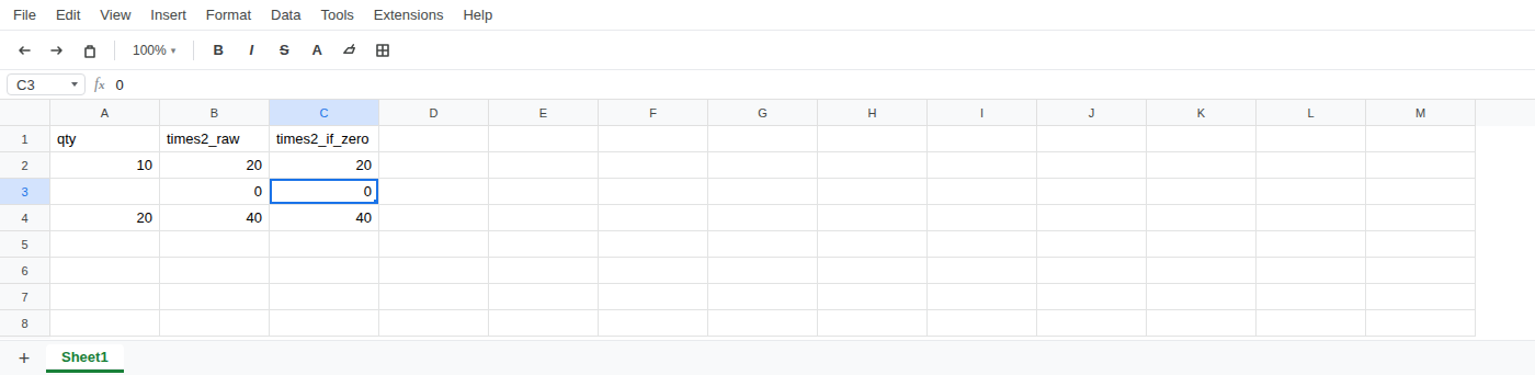
Sheet1. In A1 typeqty, B1times2_raw, C1times2_if_zero. - In A2 type
10as a number. Leave A3 empty. In A4 type20as a number. - In B2 enter
=ARRAYFORMULA(A2:A4*2). The column spills 20, then0, then 40. The middle row is 0. There is no red error triangle.
- In C2 enter
=ARRAYFORMULA(IF(A2:A4="",0,A2:A4*2)). That column is also 20,0, 40. Writing0in the IF empty branch does not make a blank row.
Leave B2 and C2 as the broken formulas so the zeros stay visible.
Second recreate — COUNT treats the 0 as a value. In F1 type count_raw. In F2 enter =COUNT(B2:B4). The cell shows 3. COUNT counts numbers. The middle 0 is a number. A3 was empty, so you might have expected 2. The spill invented a third numeric cell.
That is why the 0 is not cosmetic. Dashboards that count filled rows, charts that plot the column, and SUM of the spill all pick up the fake zeros. COUNTA(B2:B4) is also 3. The cell is not blank.
What is actually wrong
Section titled “What is actually wrong”An empty cell times 2 is treated as 0. Arithmetic in Sheets coerces a blank to zero the same way =A3*2 in a single cell would. ARRAYFORMULA just writes that 0 into every blank input row in the range. The formula is working.
Putting 0 in the IF empty branch still prints 0. IF(A2:A4="",0,A2:A4*2) tests for blank input, then deliberately stores the number zero. The cell is the number zero, not a blank. COUNT cannot tell that 0 from a real qty of zero.
A real qty of 0 (someone typed zero) is a different row. If you need to keep typed zeros and only hide empty input rows, test A2:A4="" (empty), not A2:A4=0. Empty equals 0 in math, but ="" is the blank test. =0 would also hide a legitimate zero qty.
This is not #DIV/0!. Nothing was divided. See divide by zero. This is not #VALUE! from adding the word pcs. See wrong type. This is not a spill #REF!. The cells below B2 were empty, so the array expanded. See SORT / UNIQUE spill if the formula itself is #REF!.
This is not FILTER #N/A from zero matching rows. See FILTER no match. ARRAYFORMULA did not filter. It filled.
Leave B2 and C2 as the broken formulas so the zeros stay visible.
In D1 type times2_if_blank. In D2 enter =ARRAYFORMULA(IF(A2:A4="","",A2:A4*2)). The column spills 20, a blank-looking cell, then 40.
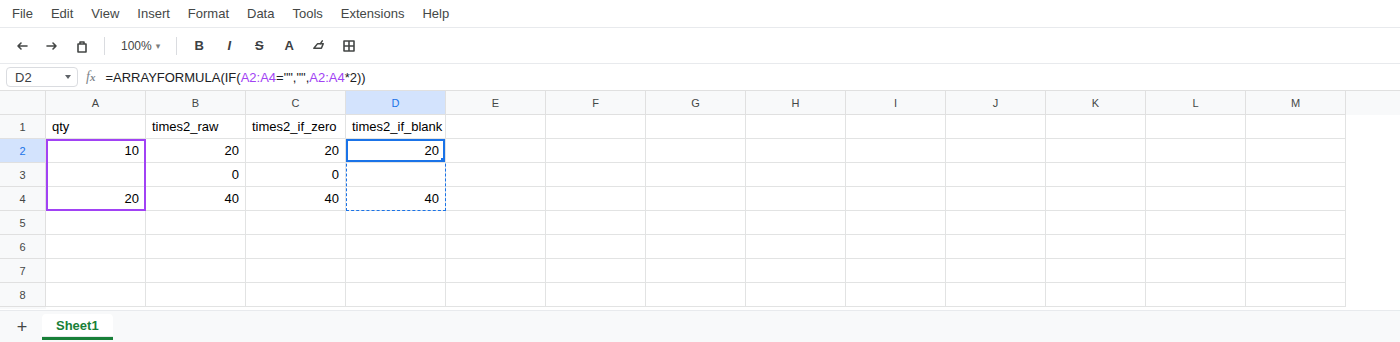
That middle cell is "", an empty string, not a truly empty cell. COUNT(D2:D4) returns 2. COUNTA(D2:D4) still returns 3 because an empty string is not a blank cell. If you need COUNTA to ignore those rows, keep the input column empty and count A2:A4, or count only numbers in the output (COUNT).
Do not use 0 as the empty-row result. Do not wrap the formula in IFERROR to “clean” the column. There is no error to catch.
If a qty cell is blank, keep the output blank with "". 0 is a value.