

Circular dependency detected in Google Sheets
Updated
A formula that points at its own cell lands as #REF!. Sheets cannot finish the value. That is a loop, not a missing range. Two cells that point at each other are the same error. A SUM whose range includes the SUM cell is the same error. The tooltip mentions iterative calculation. Do not turn that setting on for this page.
Recreate it on a blank sheet
Section titled “Recreate it on a blank sheet”- Open a blank spreadsheet. In A1 type
10. - In A2 enter
=A1+A2. The cell shows#REF!. The tooltip is Circular dependency detected. To resolve with iterative calculation, see File > Settings.
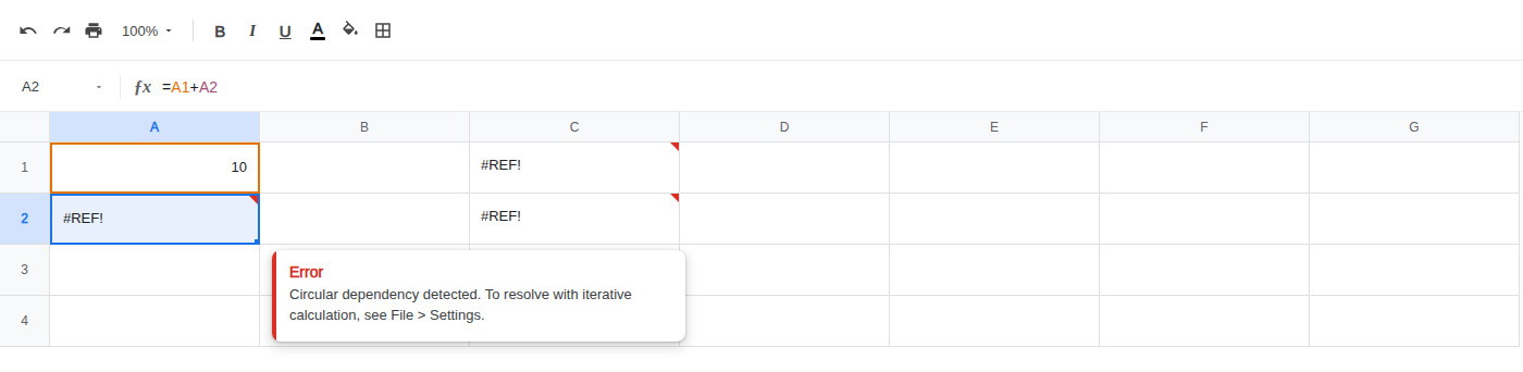
Leave A2 as the broken formula. Read the formula bar. It still says =A1+A2. The names are intact. The cell cannot finish because one of those names is A2 itself.
Second recreate — two cells. In C1 enter =C2. In C2 enter =C1. Both cells show #REF!. Neither formula names itself. Each formula depends on the other, so neither can start. That is still a circular dependency. It is not a different error value. Leave C1 and C2 broken.
Third recreate — a SUM that includes itself. In E1 type 10. E2 20. In E3 enter =SUM(E1:E3). The cell shows #REF!. The tooltip is the same circular message. E3 asked for a total of E1:E3, and E3 is inside that range. This is the loop you get on a total row when the range was dragged one cell too far. Leave E3 broken.
What is actually wrong
Section titled “What is actually wrong”=A1+A2 in A2 asks A2 for a value that includes A2. Sheets would need A2’s result in order to compute A2. That never finishes, so the cell is #REF!. The formula parsed. A1 is a real 10. There is nothing to Allow access to.
C1 =C2 and C2 =C1 is the same cause split across two cells. C1 is waiting on C2. C2 is waiting on C1. You will not see a self-name in either formula bar. You have to follow the reference. Three or four cells in a ring (F1=F2, F2=F3, F3=F1) behave the same way. Every cell in the cycle shows #REF!.
=SUM(E1:E3) in E3 is the self-ref hiding inside a range. People miss it because E3 does not appear as a single operand. The range is the operand. If the formula cell sits inside the range, it is a loop. =SUM(E:E) written anywhere in column E is the same trap.
Iterative calculation is the wrong fix here. The tooltip points at File > Settings. Under Calculation you can turn Iterative calculation on, set a max number of iterations, and set a threshold. That feature exists for models that intentionally converge — a value that is defined as feeding on its previous approximation. =A1+A2 in A2 is not that model. If you turn the setting on, Sheets stops reporting #REF! and writes a number instead. For =A1+A2 that number is not “A1 plus A2.” A2 has no independent value. Each iteration adds A1 onto whatever A2 held last time, so the cell grows (or sits on an arbitrary seed) until the iteration cap. You have not computed a total. You have hidden the loop. The two-cell pair and the self-SUM behave the same way: a number appears, and it is not the number the formula was written to mean.
Turn iterative calculation off if you switched it on while reading the tooltip. Then fix the references. If you actually need a running total, point at the previous row (=E2+D3 in E3) or at a range that stops above the formula (=SUM(E1:E2)). That is a chain, not a cycle.
This is not a deleted reference. After a delete, #REF! appears inside the formula bar (=A1+#REF!). See after you delete. A2 still names A1 and A2. C1 still names C2. E3 still names E1:E3.
This is not a SORT or UNIQUE spill hitting a blocked cell. That tooltip is Array result was not expanded. See SORT / UNIQUE spill.
This is not VLOOKUP asking for a column the range does not have. See VLOOKUP bad index. This is not IMPORTRANGE waiting for Allow access.
How to find the loop
Section titled “How to find the loop”Start at any #REF! whose tooltip says Circular dependency detected. Open the formula bar. Do not hunt for a deleted name. The names are still there.
If the formula names its own cell (=A1+A2 sitting in A2, =SUM(E1:E3) sitting in E3, =A2 sitting in A2), you have the loop. Change that reference.
If it does not name itself, click each address in the formula (Sheets colors them). Open those cells. If one of them names the first cell, you have a two-cell loop. Keep walking if you have to. Named ranges can hide the same cycle: a name that includes the formula cell is still a self-ref. Edit the name, or stop using it in that cell.
A whole column in a SUM, AVERAGE, or COUNTA that lives in that column is the usual “I cannot see A2 in the formula” case. Narrow the range so it ends on the last input row, not on the formula row.
Sheets does not give you Excel’s status-bar jump list for circular references. The #REF! cells are the list. Walk them from the formula bar.
Remove the self-reference. Change A2 to =A1. The cell shows 10.
Leave C1 and C2 as they are so the two-cell loop stays #REF! on the sheet.
Change E3 to =SUM(E1:E2). The cell shows 30. Do not leave E3 as =SUM(E1:E3).
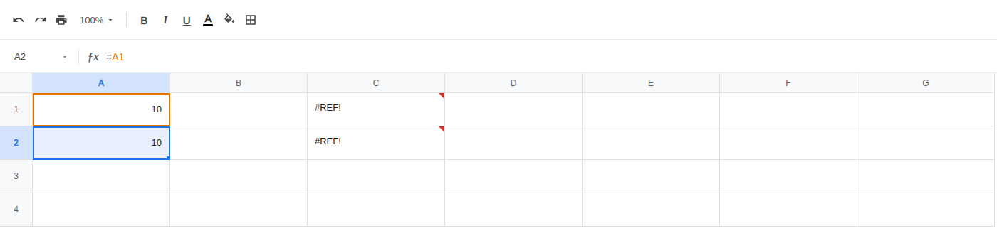
Point the formula at cells that do not depend on this cell. Do not wrap the #REF! in IFERROR. Do not turn iterative calculation on to make the error disappear. The loop is the bug. Break the loop.