The wrong AGGREGATE function_num or option still includes errors or hidden rows

AGGREGATE(function_num, options, range) is an Excel function. function_num picks the math: 9 is SUM, 1 is AVERAGE, 4 is MAX. options picks what to skip, and the codes are easy to swap. Option 0 ignores nested SUBTOTAL and AGGREGATE results and still chokes on #DIV/0!. Option 6 ignores errors and still includes rows you hid by hand, and it does not ignore nested subtotals. Option 1 is AVERAGE, so a “total” comes back as a mean. Google Sheets has no AGGREGATE. The same formula is #NAME? there.

Sheets’ skip for hidden rows is SUBTOTAL hidden rows. Sheets’ skip for nested subtotals is nested SUBTOTAL. An unknown function name is unknown function. Keep the Google Sheets UI in English when you open the file in Sheets. Sheet Error is not Microsoft and not Google.

Recreate it on a blank sheet

1. You want Excel for the option codes and Google Sheets for the #NAME?. In Excel, in A1 type qty. A2 type 10. A3 type 20. In A4 enter =1/0. A4 is #DIV/0!. A5 type 30. The numeric sum, ignoring the error, is 60. The average of those three numbers is 20.

Option 0 still returns the error. In C1 type opt0. In C2 enter =AGGREGATE(9,0,A2:A5). Function 9 is SUM. Option 0 ignores nested SUBTOTAL and AGGREGATE only. There is no nested subtotal here, and there is an error. C2 is #DIV/0!. Leave C2 broken. Option 0 did not mean “ignore problems.”

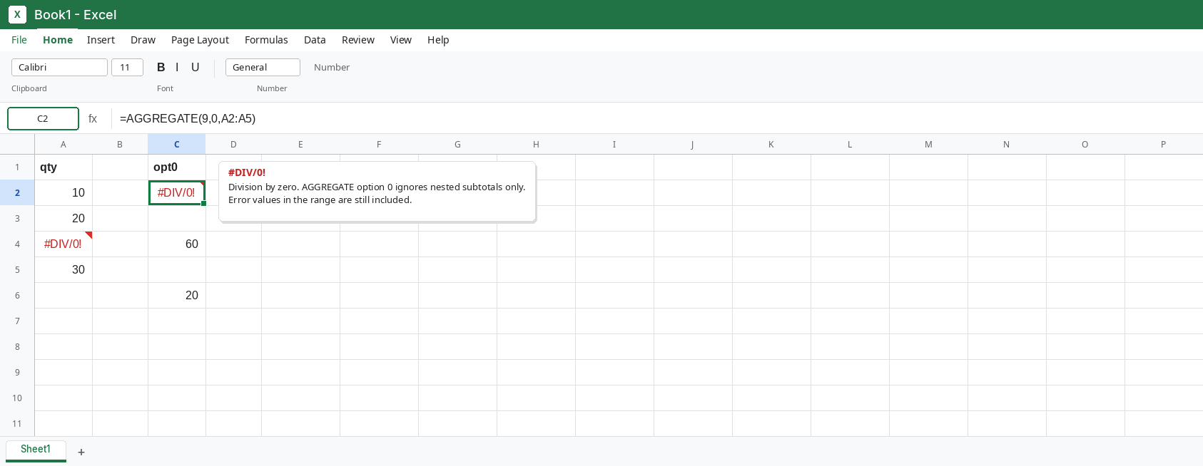
Option 6 ignores the error and is SUM. In C4 enter =AGGREGATE(9,6,A2:A5). C4 is 60. Option 6 ignores error values. It does not ignore hidden rows, and it does not ignore nested subtotals. This is the control for “sum, skip errors.”

Function 1 is AVERAGE. In C6 enter =AGGREGATE(1,6,A2:A5). C6 is 20. Same option 6, function_num 1. The cell looks like a small total. It is the mean of 10, 20, and 30. Leave C6 as 20 next to C4’s 60.

Hide a row. Hide row 5 (the 30) with the row header, Hide. C4 stays 60. Option 6 still sees the hidden row. In C8 enter =AGGREGATE(9,7,A2:A5). Option 7 ignores hidden rows and errors. C8 is 30 (10+20 only) while row 5 stays hidden. Unhide row 5 when you are done reading C8, or leave it hidden with C4 at 60 and C8 at 30.

The option families. 0 through 3 ignore nested SUBTOTAL and AGGREGATE. 4 through 7 do not. 6 is “errors only.” 5 is “hidden rows only,” so a #DIV/0! in the range still breaks a sum. 3 ignores hidden rows, errors, and nested subtotals together. A code from the wrong family still includes the thing you meant to drop.

The same formulas in Google Sheets. Open this workbook in Google Sheets, or type =AGGREGATE(9,6,A2:A5) on a blank Sheet with the same numbers. The cell is #NAME?. Sheets does not have the function. The tooltip names AGGREGATE. The option code never runs. See unknown function.

Leave the Excel C2 as #DIV/0! if you are in Excel. Leave the Sheets cell as #NAME? if you are in Sheets.

What is actually wrong

• function_num and options are both small integers, and they are not interchangeable. 1 in the first slot is AVERAGE. 1 in the second slot means “ignore hidden rows and nested subtotals.” Reading the arguments backwards changes the math and the skip list.
• Option 0 is the nested-subtotal skip, which is also what SUBTOTAL does in Sheets. It is not an error skip. One #DIV/0! still ruins the sum.
• Options 4 to 7 are the ones that can ignore errors or hidden rows without ignoring nested subtotals. A grand total written with option 6 over a column that contains category SUBTOTAL rows will add those category totals back in. See nested SUBTOTAL for the Sheets version of that double count.
• Hidden rows and filtered rows are not the same switch in every function. In Excel, AGGREGATE options that mention hidden rows are how you drop them. In Sheets, SUBTOTAL 9 versus 109 is that switch, and neither code ignores #DIV/0!. See SUBTOTAL hidden rows.
• Pasting the Excel formula into Sheets does not approximate it. #NAME? means the name was not recognized. The numbers in the arguments are irrelevant until the function exists.

This is not a Sheets calculation limit. The formula did not start.

Fix

Leave one broken sample: Excel C2 as #DIV/0!, or the Sheets #NAME?, so you can see which product you are in.

In Excel, pick the code pair you can point at. Sum, ignore errors, include hidden rows: =AGGREGATE(9,6,A2:A5) is 60 with row 5 visible. Sum, ignore errors and hidden rows: option 7. Sum, ignore errors and nested subtotals: option 2. Average is function 1, not a different option. After you change a code, compare the cell to 60 or 20 on this sample before you trust a larger range.

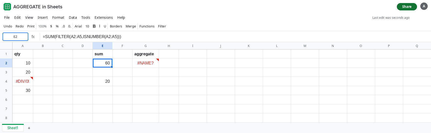
In Google Sheets, do not call AGGREGATE. For a sum that skips errors and text, in E2 enter =SUM(FILTER(A2:A5,ISNUMBER(A2:A5))). E2 is 60. ISNUMBER drops the #DIV/0!. For an average, =AVERAGE(FILTER(A2:A5,ISNUMBER(A2:A5))) is 20. For hidden rows, use SUBTOTAL with 109 on a range that does not contain errors, or filter the errors first. One Sheets function does not take a function_num and an options code. See SUBTOTAL hidden rows and nested SUBTOTAL.

If the tooltip says #NAME? and the name is AGGREGATE, you are in Sheets. If Excel returns #DIV/0! and the option is 0 or 5, errors are still included. If the result is about a third of the sum you expected, function_num is probably 1.