XLOOKUP search_mode -1 returns the last duplicate, which is not the latest date

XLOOKUP’s sixth argument is search_mode. -1 walks the lookup range from bottom to top and returns the first hit it finds, which is the last duplicate on the sheet. It does not sort by a date column. If the lower 101 is an older sale than the upper 101, -1 returns the older bin. The default, first-to-last, returns the upper row. Neither result is #N/A. The fifth argument -1 is match_mode (exact or next smaller), not this search. Putting -1 in the missing-value slot does not search from the bottom at all.

Binary search (2 and -2) on unsorted data is XLOOKUP search_mode. Wildcard and next-larger are XLOOKUP match_mode. A real miss is XLOOKUP #N/A. Keep the Google Sheets UI in English. Sheet Error is an independent formula-error library, not a Google product.

Recreate it on a blank sheet

1. Open a blank spreadsheet. In A1 type sku, B1 bin, C1 sold. A2 101, B2 Old, C2 =DATE(2024,3,1). A3 102, B3 Other, C3 =DATE(2024,1,1). A4 101, B4 New, C4 =DATE(2024,1,15). Format C2:C4 as Date. Sku 101 is on two rows. The March date is on the first 101. The January date is on the last 101. The row labeled New is not the latest sale.

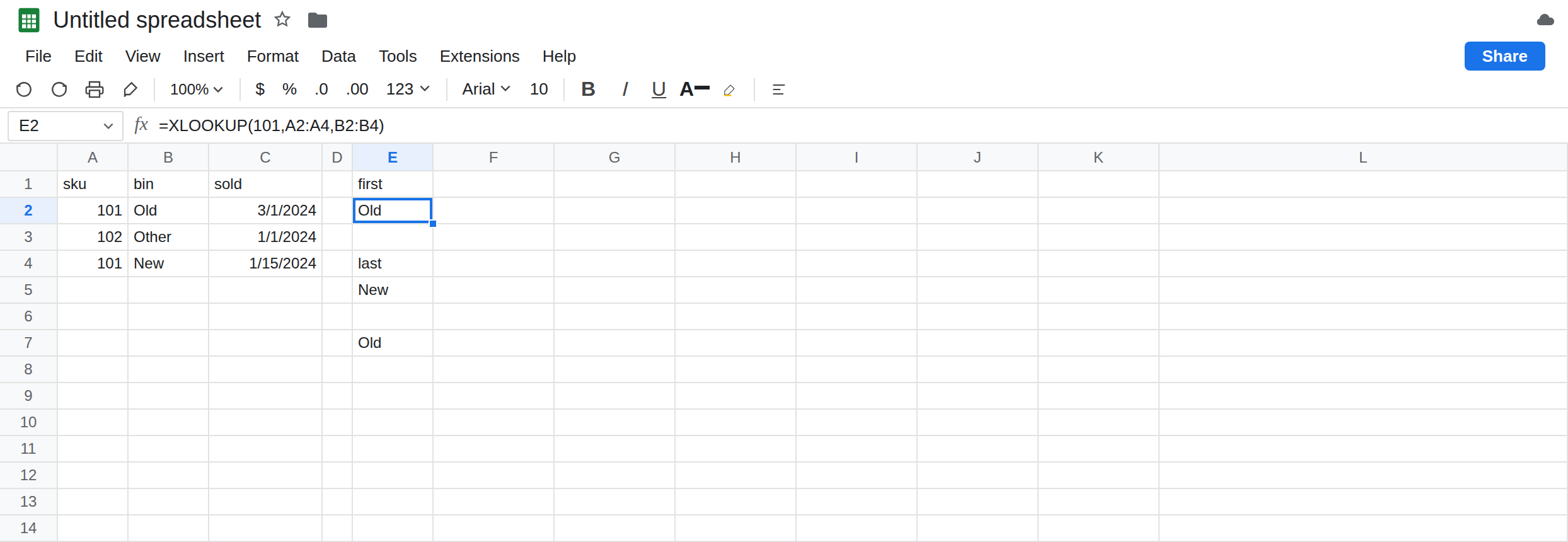
First hit, the default. In E1 type first. In E2 enter =XLOOKUP(101,A2:A4,B2:B4). E2 is Old. Search mode 1 is the default: top to bottom. The March row wins because it sits higher, not because March is later. Leave E2 as Old.

Last hit. In E4 type last. In E5 enter =XLOOKUP(101,A2:A4,B2:B4,,0,-1). The fourth argument is empty (if_not_found omitted), the fifth is 0 (exact), the sixth is -1 (bottom to top). E5 is New. That bin’s date is 15 January, which is before 1 March. You asked for the last row, and you got it. You did not ask for the maximum date. Leave E5 as New.

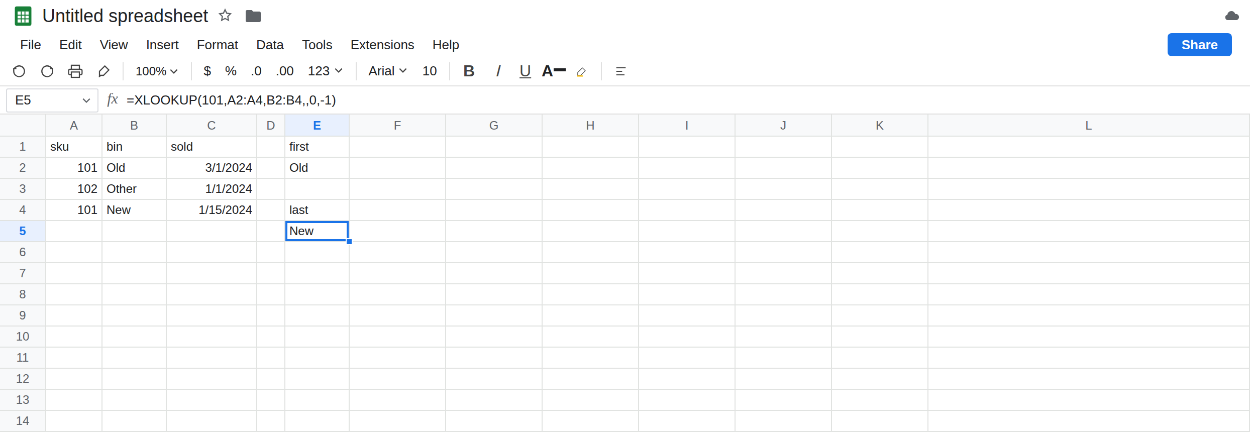
-1 in the wrong slot. In E7 enter =XLOOKUP(101,A2:A4,B2:B4,-1). That -1 is if_not_found. The sku exists, so the missing-value is never used. E7 is Old, same as E2. The search is still top to bottom. In E8 enter =XLOOKUP(101,A2:A4,B2:B4,,-1). That -1 is match_mode: exact or next smaller. 101 exists, so the exact row wins and you still get a first-hit story (Old), not New. Looking up a key that is not there is the case that separates them. In E9 enter =XLOOKUP(100,A2:A4,B2:B4,,-1). The keys are 101 and 102. Nothing is less than or equal to 100, so E9 is #N/A. That #N/A is next-smaller failing, not a bottom-to-top scan. Leave E7 as Old so a misplaced -1 stays visible. See XLOOKUP match_mode.

A true miss still misses from the bottom. In E11 enter =XLOOKUP(999,A2:A4,B2:B4,"none",0,-1). E11 is none. Searching last-to-first does not invent a row for 999. Without "none", that call is #N/A. That miss is XLOOKUP #N/A. Leave E11 as none.

Every bin, if you need both. In G2 enter =FILTER(B2:B4,A2:A4=101). G2 spills Old and New. One XLOOKUP will not. Leave G2 as two rows.

Leave E5 as New. Leave E2 as Old. Leave E7 as Old.

What is actually wrong

• search_mode -1 is an order of scanning, not a sort. “Last” means the last row in the range as it is laid out. If the sheet is not sorted by date, the last row is not the latest sale. E5 versus C2 is that layout.
• The sixth argument is not the fifth, and not the fourth. You have to leave commas for the slots you skip. ,,0,-1 is exact match, then last-to-first. -1 alone after the result range is a missing-value of negative one, and only a miss would show it.
• if_not_found does not run when a duplicate is found. E5 returns New even if you pass "none". "none" is for 999, which is E11.
• Binary mode is not “a faster -1.” Mode 2 requires ascending data and can return #N/A or the wrong row when the skus are 101, 102, 101. That recreate is XLOOKUP search_mode. This page does not use mode 2.
• A two-column result still spills sideways. Last-to-first does not change that. A blocked neighbor is XLOOKUP return range.

This is not VLOOKUP wrong row. VLOOKUP’s approximate match is the fourth argument TRUE. XLOOKUP defaults to exact. E5 is exact, twice, and the scan direction picked the second exact hit.

This is not text versus number. Both 101s are numbers. See VLOOKUP no match if one of them is text and E5 is #N/A instead of New.

Fix

Leave E5 as the last row and E7 as the misplaced -1.

You wanted the first bin. Keep E2. Do not pass -1.

You wanted the last row on purpose. Keep E5, and label the column last row, not latest. If a new 101 is appended, E5 moves. That is the feature.

You wanted the latest date. XLOOKUP will not maximize C. Sort the matching rows, or take the max date first. One pattern: =XLOOKUP(MAXIFS(C2:C4,A2:A4,101),C2:C4,B2:B4). The max date for sku 101 is 1 March, and the bin is Old. If two rows share that date, you are back to first versus last on the date column. FILTER plus SORT is the list when you need every row. G2 is the unsorted list of bins.

Write the commas. Copy E5’s shape when you mean last-to-first: empty missing-value, 0, then -1. Copy E11’s shape when the sku might be absent.

Do not wrap E5 in IFERROR. New is a real bin. See IFERROR vs IFNA.

If -1 returned the bottom duplicate, it was the sixth argument and the result is the last row, not the latest date. If -1 seemed to do nothing on a sku that exists, it is in the fourth or fifth slot. If the cell is #N/A and the sku is visible twice, check text versus number and mode 2 on the other page. If the sku is not in the column, pass if_not_found.

Last row vs first row vs the wrong -1

Default XLOOKUP of 101 is Old (1 March). ,,0,-1 is New (15 January). -1 as if_not_found is still Old. match_mode -1 is not the bottom scan. 999 is still missing. The latest sale is the max date, which on this sheet is the first row, not the last.