Excel spilled arrays become static values when the file opens in Google Sheets

Updated 2026-09-29

Excel’s dynamic arrays spill from one formula. FILTER, UNIQUE, SORT, and SEQUENCE can fill the cells below the anchor, and A1# refers to that spill. Google Sheets has its own spilling formulas. It does not keep Excel’s spill reference. When you open or import the .xlsx, check the formula bar. If the cells under the anchor are numbers and the bar is empty, those cells are values. Editing the source will not grow the block. The picture survived. The array did not.

Sheet Error is not Microsoft and not Google. Keep the Google Sheets UI in English. A blocked spill inside Sheets (#REF!, Array result was not expanded) is array result was not expanded. This page is the file that used to spill in Excel.

Recreate it on a blank sheet

You need Excel for the first half and Google Sheets for the second. In Excel, in A1 type sku. A2 101. A3 102. A4 101. In C1 type spill. In C2 enter =UNIQUE(A2:A4). C2 spills 101 and 102. C3 is part of the spill. The formula lives in C2. Select C3. The formula bar shows it belongs to the spill (Excel shows the formula as part of that array, and a reference like =C2# in another cell would point at the whole spill). That block is the control in Excel.

Save and open in Sheets. Save the workbook as .xlsx. In Google Sheets, File → Import → Upload, choose the file, and import it (replace the current sheet, or open the upload as a new spreadsheet). Go to the cell that shows 101 under the unique list.

Read the formula bar, not the paint. Click the top cell of that list, then the cell under it. You are looking for one of these, and you should believe the bar:

The top cell contains a Sheets formula such as =UNIQUE(A2:A4) and the cell under it is empty in the formula bar while still showing 102. Sheets is spilling. Change A3 and see whether the spill follows. If it does, this file is fine. Stop.
The top cell and the cell under it both show values, and the formula bar is empty on both. The spill was flattened to values. Change A2 from 101 to 999. The unique list does not change. Leave it that way. That frozen list is the recreate.
A cell contains =C2# or another # spill reference. Sheets does not use that operator. The cell errors (a parse error or #NAME? / #ERROR!, depending on the import). The # is Excel. Leave that cell broken.

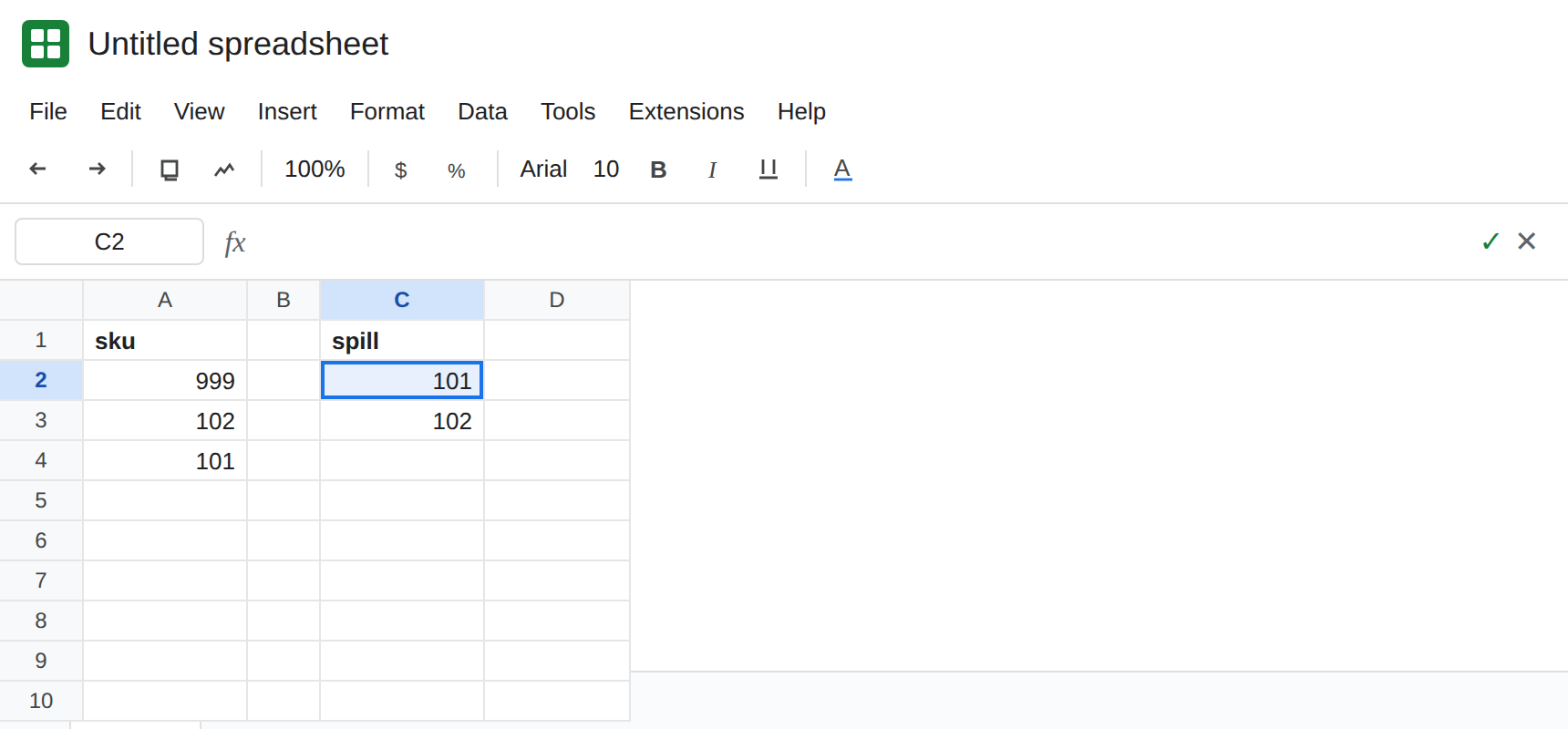
Google Sheets after importing an xlsx. The unique list shows 101 and 102. The formula bar on those cells is empty. A2 is 999 and the list did not change. No UNIQUE formula remains.

FILTER behaves the same way. If the Excel file used =FILTER(A2:A4,A2:A4<>"") and the imported block is values, editing A2 will not change the filter output. The test is always the formula bar on the anchor and on the next cell. Do not assume every function dies. Some anchors keep a formula Sheets understands. The ones that matter are the ones whose bar is empty.

This is not array result was not expanded. That #REF! means a Sheets formula tried to spill and a cell was in the way. A static import does not try.

What is actually wrong

Excel stores a dynamic array on the anchor and paints the spill. Sheets has to translate that package on import. When the translator keeps calculated values and drops the formula, the grid looks finished. It will not expand when rows are added in column A.
The # spill operator is Excel syntax. =C2# is not a named range and not a Sheets function. Rewriting it as text will not reconnect the block.
A formula Sheets shares with Excel (UNIQUE, FILTER, SORT, SEQUENCE) can survive on the anchor. Survival is something you verify per cell. A screenshot of the numbers is not the verification.
Copying the spill in Excel and pasting into Sheets with the default paste also pastes values if you copied the results. Paste formulas only when the source cell actually holds a formula Sheets can parse. Locale separators can still break it. See locale parse error.
The import does not create a live link back to the .xlsx. Later saves in Excel do not update the Sheets file unless you import again, which can flatten the array again.

Fix

Leave one imported block as values so you can see that editing A2 does nothing.

Type the Sheets formula again on a clear range. In E1 type live. Clear E2:E5. In E2 enter =UNIQUE(A2:A4). E2 spills the current skus. Change A2. The spill follows. That is the control inside Sheets. =FILTER(A2:A4,A2:A4<>"") is the same idea when the Excel formula was FILTER.

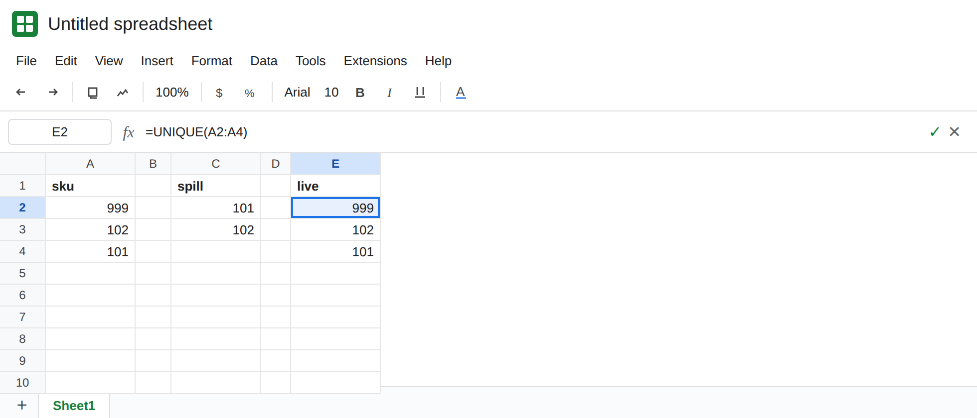
E2 selected. Formula bar shows =UNIQUE(A2:A4). E2 spills the current skus and updates when A2 changes. The imported block still shows the old 101 and 102 as values with an empty formula bar.

Replace a # reference with the spill formula or with a normal range. If a cell says =C2#, put =UNIQUE(A2:A4) or point at the range the spill occupies after you have recreated it. Do not leave the hash.

If the anchor already has a working Sheets formula, do not paste values over it. The import succeeded for that cell. Add new source rows inside the range the formula names (A2:A4 will not see A5 until you extend it or use an open range you actually want).

Do not wrap the static block in IFERROR. There is no error to hide. The risk is a silent stale list. See IFERROR hides cause.

If the formula bar is empty, the spill is a snapshot. Enter UNIQUE or FILTER again. If the bar shows a formula and a neighbor cell blocks the spill, you are on the #REF! overwrite page. If the bar shows a trailing #, that reference is Excel’s, not a Sheets name.