HSTACK fills the short side with #N/A, and AVERAGE of the spill is #N/A

HSTACK places arrays side by side and uses the taller height. The short array is filled with #N/A in the rows it does not have. The formula does not error. SUM and AVERAGE of that spill do. One pad cell is enough. A blank cell in a range of the same height is a blank, and AVERAGE can ignore it. #N/A is not a blank.

The name-roster version of this pad is HSTACK rows. The combined shape primer is HSTACK / VSTACK pad. This page is what the pad does to a total. Keep the Google Sheets UI in English. Sheet Error is an independent formula-error library, not a Google product.

Recreate it on a blank sheet

1. Open a blank spreadsheet. In A1 type am. A2 10. A3 20. A4 30. In C1 type pm. C2 8. C3 12. Leave C4 empty. Three morning scores. Two afternoon scores. The empty C4 is not part of the short range.

Uneven stack. Leave E2:F4 empty. In E1 type side. In E2 enter =HSTACK(A2:A4,C2:C3). The spill is three rows and two columns. E2:E4 is 10, 20, 30. F2 is 8. F3 is 12. F4 is #N/A. No error triangle on E2. Leave E2 as that spill.

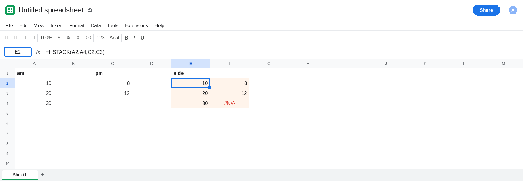
The aggregates. In H1 type avg. In H2 enter =SUM(E2:F4). H2 is #N/A. In H3 enter =AVERAGE(E2:F4). H3 is #N/A. The five scores total 80 if you add them by hand. The pad blocks both functions. Leave H2 and H3 broken.

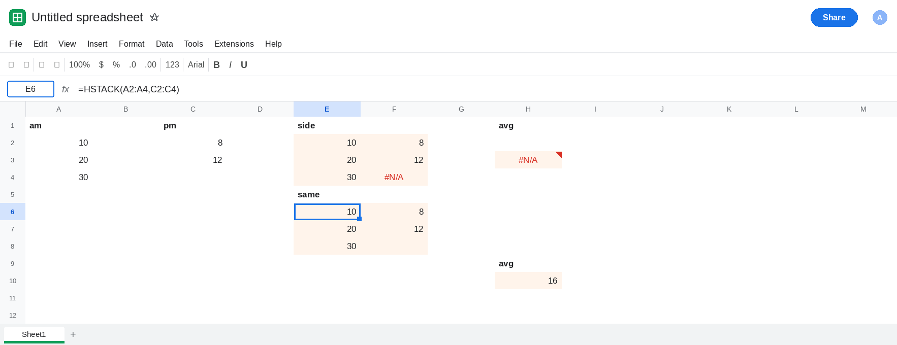
Same height, blank cell. In H5 enter =HSTACK(A2:A4,C2:C4). C4 is empty, and the range is three rows. The third afternoon cell is blank, not #N/A. In H8 enter =AVERAGE(H5:I7). H8 is 16. AVERAGE skips the blank. (10+20+30+8+12) / 5 is 16. That block is the control for “the slot exists and is empty.”

A chart of the pad. Select E2:F4. Insert → Chart. A line or column chart gaps or breaks on F4. The scores did not. The #N/A did. Details of how series treat error cells are chart error gaps. Leave the chart up if you want the gap visible. The numeric proof is H3.

Leave F4 as #N/A. Leave H3 as #N/A. Leave H8 as 16.

What is actually wrong

• HSTACK will not stop at the shorter list and will not refuse the way FILTER refuses mismatched heights. It pads. F4 is the contract. See FILTER range size for the function that errors instead.
• SUM and AVERAGE propagate #N/A. They do not drop it. H2 and H3. AVERAGE of the source pieces separately is fine: AVERAGE(A2:A4) is 20, AVERAGE(C2:C3) is 10. The failure starts when the pad is inside the range you aggregate.
• A blank in a same-height range is a different cell. H5. Passing C2:C3 because C4 “is empty anyway” is what creates F4. Include C4 when the row exists and is blank.
• IFNA can turn F4 into a blank after the fact. IFNA on a whole HSTACK also turns a real #N/A from the source into a blank. Prefer a same-height range when the missing afternoon score is “no score yet” and not “an error you meant to keep.”
• VSTACK pads width, with #N/A out to the right. That is VSTACK cols. Blank rows brought back by stacking an unfiltered range are VSTACK blank rows.

Fix

Leave E2 and H3 as the #N/A path.

Give both sides the same height. In E6 enter =HSTACK(A2:A4,C2:C4). Copy the average: in H10 enter =AVERAGE(E6:F8). H10 is 16. The third afternoon cell is blank because C4 is blank. SUM(E6:F8) is 80.

If the short list is a formula spill, pad that spill before you stack. IFNA around the short piece only: =HSTACK(A2:A4,IFNA(C2:C3,"")) still does not add a third row. IFNA replaces error values. It does not add missing rows. The height has to match first. Stack ranges that already have the same number of rows, then aggregate.

Do not wrap H3 in IFERROR and treat 0 as the average. See IFERROR vs IFNA. A zero average and a #N/A average are both the wrong reading of these five scores. 16 is the average that ignores the empty seat.

If AVERAGE of an HSTACK is #N/A and the bottom cell on the short side is #N/A, the ranges differ in height. Extend the short range with a blank, or average the two lists separately. If the bottom cell is blank and the average is a number, you are looking at a same-height stack and the pad page’s failure is already gone.