SUMIF and SUMIFS only see the top-left cell of a merged category

A merged range paints one value across several cells. Sheets stores that value in the top-left cell only. The other cells in the merge are empty. SUMIF and SUMIFS compare cells, not the painted block. A category that looks like it covers three qty rows is one label and two blanks, so the total is the first row only. Pointing the criterion argument at the blank half of a merged cell is a second miss: the criterion itself is empty, and the sum is 0. There is no error triangle. The number is simply small.

VLOOKUP on the same merge is merged cells lookup. That page is the single-key picture, including one SUMIF. This page is the criteria range, a second SUMIFS condition, and a criterion that references the wrong cell of a merge. An invisible CHAR(160) is CHAR(160) blanks. Keep the Google Sheets UI in English. Sheet Error is an independent formula-error library, not a Google product.

Recreate it on a blank sheet

1. Open a blank spreadsheet. In A1 type region, B1 status, C1 qty.

Merge the category on purpose. Select A2:A4. Format → Merge cells → Merge vertically. Type East and press Enter. The word sits across three rows. B2 open, C2 10. B3 open, C3 3. B4 hold, C4 7. A5 type West with no merge. B5 open, C5 4. East open should be 13 (10+3). East overall should be 20. The eye says so. The cells do not.

Prove the blanks. In E1 type probe. In E2 enter =A2. E2 is East. In E3 enter =A3. E3 is blank. In E4 enter =ISBLANK(A3). E4 is TRUE. =COUNTA(A2:A4) is 1.

SUMIF adds the top-left only. In G1 type sumif. In G2 enter =SUMIF(A2:A5,"East",C2:C5). G2 is 10. Rows 3 and 4 display East and are not East. Leave G2 as 10.

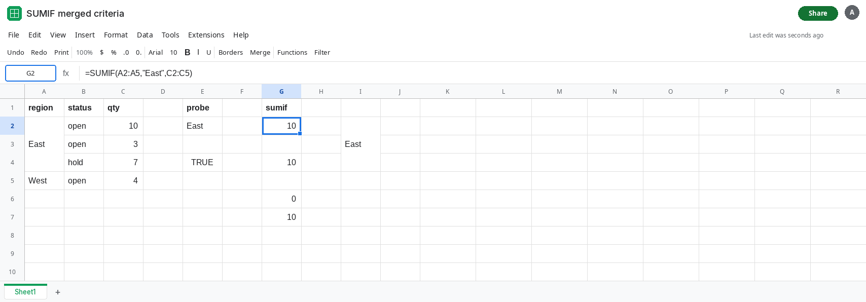
SUMIFS still misses the lower open row. In G4 enter =SUMIFS(C2:C5,A2:A5,"East",B2:B5,"open"). G4 is 10. B3 is open and C3 is 3, and A3 is blank, so the East test fails. The second condition never gets a chance to save the row. Leave G4 as 10. The unmerged West row is not the problem. =SUMIF(A2:A5,"West",C2:C5) is 4.

The criterion cell is itself a merge, and you referenced the blank half. Select I2:I4. Merge vertically. Type East in that merge. In G6 enter =SUMIF(A2:A5,I3,C2:C5). I3 is not the top-left of I2:I4. I3 is blank. The criterion is blank. G6 is 0. In G7 enter =SUMIF(A2:A5,I2,C2:C5). I2 is the top-left, so the criterion is East, and G7 is 10, the same short total as G2. Leave G6 as 0.

Leave G2 as 10, G4 as 10, and G6 as 0.

What is actually wrong

• Merge is a display. The value lives in the top-left cell. SUMIF’s criteria range is a list of cells. Blank cells do not equal East, so their qty is not added.
• A second condition does not fill those blanks in. SUMIFS requires every criterion to match on that row. A blank region fails East even when status is open.
• Referencing a merged criterion also depends on which cell you clicked. The top-left holds the word. Any other cell in the merge is an empty criterion, and an empty criterion matches empty criteria cells, not the word East. The sum goes to 0 instead of to the short 10.
• The qty cells are fine. They were not merged. Merging C2:C4 would drop 3 and 7 as well, because those values would have nowhere to live but the top-left. Unmerge before you trust either column.
• There is no triangle because nothing failed. 10 and 0 are successful sums of the cells Sheets actually stores.

This is not SUMIF text numbers. The qtys are real numbers. The labels are missing.

Fix

Leave G2, G4, and G6 broken so the short totals stay visible.

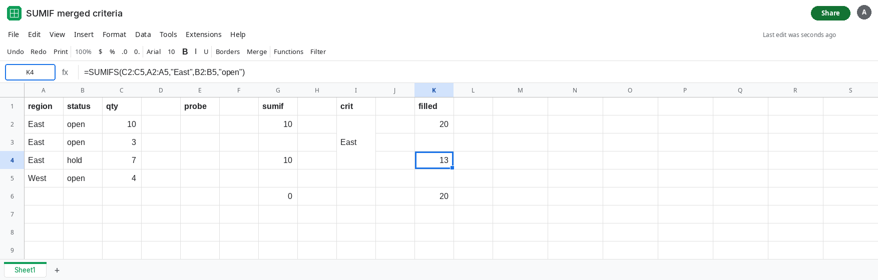
Unmerge and fill the label down. Select A2:A4. Format → Merge cells → Unmerge. A2 still says East. A3 and A4 are empty. Select A2:A4 again and use Edit → Fill → Down, or copy A2 into A3:A4. =COUNTA(A2:A4) is 3.

In K2 enter =SUMIF(A2:A5,"East",C2:C5). K2 is 20. In K4 enter =SUMIFS(C2:C5,A2:A5,"East",B2:B5,"open"). K4 is 13. In K6 enter =SUMIF(A2:A5,I2,C2:C5). K6 is 20, because the criterion is the top-left East and the criteria range is filled. Do not point K6 at I3.

If you must keep the merge for printing, do not use that painted column as a criteria range. Helper column: in M2 enter =A2 and fill down before you merge, or unmerge, fill, and merge a copy used only for display. SUMIFS should read the helper.

If G2 equals the first qty only and ISBLANK is TRUE on the next label cell, the label is merged. If G6 is 0 and the criterion’s formula bar is blank, you referenced the empty half of a merged criterion. If COUNTA on the label block equals the number of rows, the merge is gone and a short total is a real filter miss.