Fix LEFT / RIGHT / MID #VALUE! in Google Sheets (negative or non-integer length)

LEFT(text, n) takes the first n characters. RIGHT takes the last n. MID(text, start, n) takes n characters beginning at start (1-based). #VALUE! here means a length or start that is negative, or a MID start of 0. A non-integer length is usually truncated, not rejected. MID start past the end returns blank, not #VALUE!.

This page is LEFT / RIGHT / MID domain. It is not FIND / SEARCH miss (FIND #VALUE! when the needle is absent — often fed into MID). It is not SUBSTITUTE instance. Keep the Google Sheets UI in English.

Recreate it on a blank sheet

1. Open a blank spreadsheet. In A1 type lot. A2 N12E7W4 (seven characters, no hyphens).

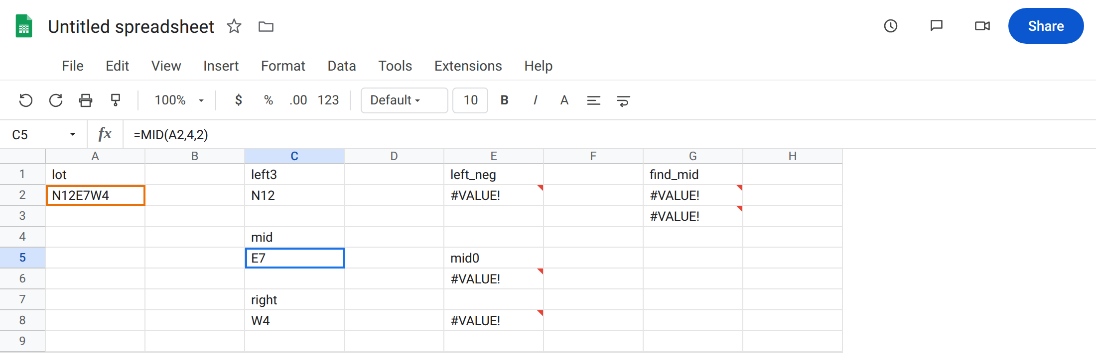
Working extracts. In C1 type left3. In C2 enter =LEFT(A2,3). The cell shows N12. In C4 type mid. In C5 enter =MID(A2,4,2). The cell shows E7. In C7 type right. In C8 enter =RIGHT(A2,2). The cell shows W4. Those three are the control.

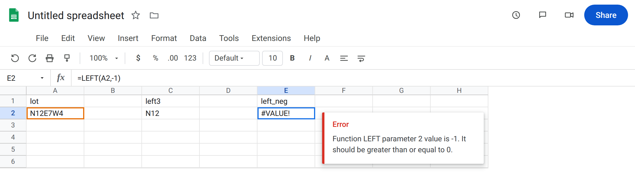
LEFT of a negative length. In E1 type left_neg. In E2 enter =LEFT(A2,-1). The cell shows #VALUE!. Length must be ≥ 0. Leave E2 broken.

MID start 0. In E5 type mid0. In E6 enter =MID(A2,0,2). The cell shows #VALUE!. start is 1-based. 0 is not “from the beginning.” Leave E6 broken.

MID start negative. In E8 enter =MID(A2,-1,2). #VALUE!. There is no from-the-end MID. Leave E8 broken.

FIND feeding a 0 into MID. In G1 type find_mid. In G2 enter =FIND("-",A2). A2 has no hyphen. G2 is #VALUE!. In G3 enter =MID(A2,FIND("-",A2)+1,2). #VALUE! again: FIND failed, so MID never got a start. Leave G2 and G3 broken. The lot is fine. The hyphen is missing. That FIND primer is FIND / SEARCH miss.

Start past the end (not this error). In I1 type past. In I2 enter =MID(A2,20,2). The cell is blank, not #VALUE!. Legal start, nothing to copy. Leave I2 blank so you do not treat empty as an error.

Truncation. In I4 enter =LEFT(A2,3.9). The cell shows N12. 3.9 becomes 3. Not #VALUE!. Negative is the refusal; fractions usually are not.

Leave E2, E6, E8, and G3 broken. Leave C2 / C5 / C8 as working extracts.

What is actually wrong

• Lengths below 0 are #VALUE!. LEFT(A2,0) is an empty string (legal). LEFT(A2,-1) is not.
• MID start must be ≥ 1. 0 and negatives fail. RIGHT has no start argument; a negative length on RIGHT fails the same way as LEFT.
• The common production bug is MID(...,FIND(...)+1,...) when FIND is #VALUE!. G3 is that cascade. Fix FIND (or wrap it) before you blame MID.
• Non-integers are truncated toward zero for these functions. 3.9 → 3. That can silently shorten a code. It is not the red triangle on this page.
• MID with a huge start returns "". Empty is not #VALUE!. Do not wrap I2 in IFERROR looking for an error that is not there.

This is not SUBSTITUTE(...,0) instance #VALUE!. See SUBSTITUTE instance. Different argument, same token.

This is not REGEXEXTRACT #N/A. See REGEX no match. MID does not run a pattern.

This is not generic 10 + pcs. See wrong type. A2 is already text.

Fix

Leave E2, E6, E8, and G3 broken.

Use 1-based starts and non-negative lengths. Keep C5: =MID(A2,4,2). First three: keep C2. Last two: keep C8.

If FIND builds the start: confirm the delimiter exists. In G5 enter =IFERROR(MID(A2,FIND("-",A2)+1,2),"") only when a missing hyphen should print blank. Prefer IF(ISNUMBER(SEARCH("-",A2)),MID(...),"") so #REF! elsewhere still shows. See IFERROR vs IFNA. IFNA will not catch #VALUE!.

Do not pass 0 to mean “from the left.” That is LEFT, or MID(A2,1,n).

If #VALUE! and the formula is LEFT/RIGHT/MID with a negative or MID(...,0,...), this is the page. If #VALUE! and you see FIND/SEARCH in the bar, fix the miss first. If the cell is blank with MID and a large start, there is no error to wrap.

MID start 0 vs FIND cascade vs blank past end

MID(A2,0,2) is an illegal start (E6). Direct.

MID(A2,FIND("-",A2)+1,2) is a FIND miss (G3). Indirect. Same #VALUE!. Read the inner function.

MID(A2,20,2) is blank (I2). Past the end is empty, not red. Do not copy an IFERROR from E6 onto I2.