QUERY avg of text-looking numbers is not the average of the digits you see

avg in QUERY averages a numeric column. A qty that looks like 10 and is stored as text is not a number. When text is the column type, avg is #VALUE! and the tooltip names AVG_SUM_ONLY_NUMERIC. When the column is numeric and the text cells are the minority, QUERY drops those cells as null and averages the real numbers only. A column of real zeros plus left-aligned 10 and 30 returns 0. The 10 and the 30 never entered the average. The sheet still shows those digits.

sum of a mixed column is QUERY GROUP BY. Row-wise + is QUERY select add. Keep the Google Sheets UI in English. Sheet Error is an independent formula-error library, not a Google product. Locale United States.

Recreate it on a blank sheet

1. Open a blank spreadsheet. In A1 type sku, B1 qty. A2 101. In B2 type '10 (leading apostrophe). A3 102. In B3 type '20. A4 103. In B4 type '30. All three qtys are text. ISNUMBER(B2) is FALSE. They sit left-aligned unless the column format forces the other side. The apostrophe is visible in the formula bar, not in the cell.

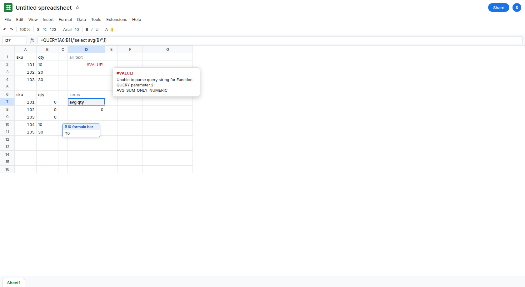
avg when the column is text. In D1 type all_text. In D2 enter =QUERY(A1:B4,"select avg(B)",1). D2 is #VALUE!. The tooltip starts Unable to parse query string for Function QUERY parameter 2 and names AVG_SUM_ONLY_NUMERIC. There is no average of 20. Leave D2 broken. This is the same aggregate contract as QUERY GROUP BY. It is not a silent zero.

The zero you get when the text is dropped. In A6 type sku, B6 qty. A7 101, B7 0 as a real number. A8 102, B8 0 as a real number. A9 103, B9 0 as a real number. A10 104. In B10 type '10. A11 105. In B11 type '30. Three real zeros, two text qtys. Text is not the majority. In D6 type zeros. In D7 enter =QUERY(A6:B11,"select avg(B)",1). The spill shows 0. ISNUMBER(B10) is FALSE. The 10 and the 30 were not averaged. The three zeros were. Leave D7 as 0.

What the digits would have averaged. In F6 type wanted. In F7 enter =AVERAGE(10,30). F7 is 20. That is the average of the two text qtys if they had been numbers, with the placeholder zeros left out. D7 is not F7. Leave both.

A sheet average of the text is the same miss. In F1 enter =AVERAGE(B2:B4). F1 is #DIV/0!. AVERAGE skips text and then has nothing to divide by. See divide by zero. D2 is the query-language version of “these are not numbers,” with a different tooltip. N(B2) is 0, which is how a later formula turns the text into a real zero and corrupts the average. See N() text to 0.

What is actually wrong

• QUERY types the column, then avg requires a number type. Three apostrophe qtys make a text column. D2’s tooltip is AVG_SUM_ONLY_NUMERIC. The digits in the cells are not a defense.
• A numeric column drops minority text as null. D7’s column has three real numbers, all 0, so the type is numeric and the average of those numbers is 0. B10 and B11 do not pull it toward 20. A blank-looking result and a displayed 0 are different. D7 is a real 0.
• The leading apostrophe is how a csv or a hand edit forces text. See CSV text vs number and CSV leading apostrophe. VALUE is a sheet function. It is not a flag inside the query string.
• avg(B) is not AVERAGE of the painted digits, and it is not sum(B)/count(B) once text has been dropped. count(B) counts non-null values in the query language, which is a different set from the rows you can see.

This is not QUERY no rows. D7 returned a row. The row is the wrong average.

Fix

Leave D2 as #VALUE!. Leave D7 as 0.

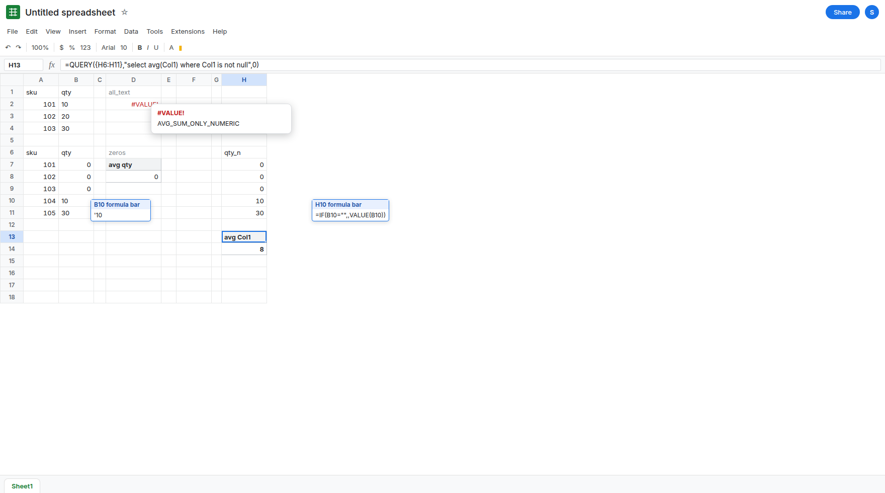
Convert, then average. In H6 type qty_n. In H7 enter =IF(B7="",,VALUE(B7)) and fill H7:H11. H7:H9 are 0. H10 is 10. H11 is 30. In H13 enter =QUERY({H6:H11},"select avg(Col1) where Col1 is not null",0). The result is 8, the average of 0, 0, 0, 10, and 30. The array uses Col1. See Col1 vs A.

Average only the qtys you meant, after they are numbers. If the zeros were placeholders and the question was the average of 10 and 30, drop them in the helper (=IF(B7=0,,VALUE(B7)) only where 0 is not a real qty) and average the rest. F7’s 20 is that question. Do not drop zeros that are real measurements.

Do not wrap D2 in IFERROR(...,0). You would turn the tooltip into a fake average of zero. See IFERROR vs IFNA. Do not run N down the column to “make avg work.” Text becomes 0 and joins D7’s average.

If avg is #VALUE! and the tooltip names AVG_SUM_ONLY_NUMERIC, the column is text. If avg is 0 while left-aligned digits sit in the same column, those digits were null to the aggregate. VALUE them, then average the helper.