Fix HSTACK / VSTACK errors in Google Sheets (mismatched sizes or #N/A padding)

HSTACK glues arrays side by side. VSTACK glues them top to bottom. When the pieces are not the same height (HSTACK) or the same width (VSTACK), Sheets still returns an array. The holes are #N/A. That is padding, not a lookup miss. A hard size error on FILTER is a different function.

This page is HSTACK / VSTACK shape. It is not FILTER range size (condition height ≠ data height; tooltip FILTER has mismatched range sizes). It is not FILTER no match (equal heights, zero rows). It is not what #N/A means as a VLOOKUP primer. Keep the Google Sheets UI in English.

Recreate it on a blank sheet

1. Open a blank spreadsheet. In A1 type morning. A2 Kim. A3 Omar. A4 Priya. Three names. In C1 type afternoon. C2 Lee. C3 Sam. Two names. Leave C4 empty on purpose. The afternoon roster is shorter.

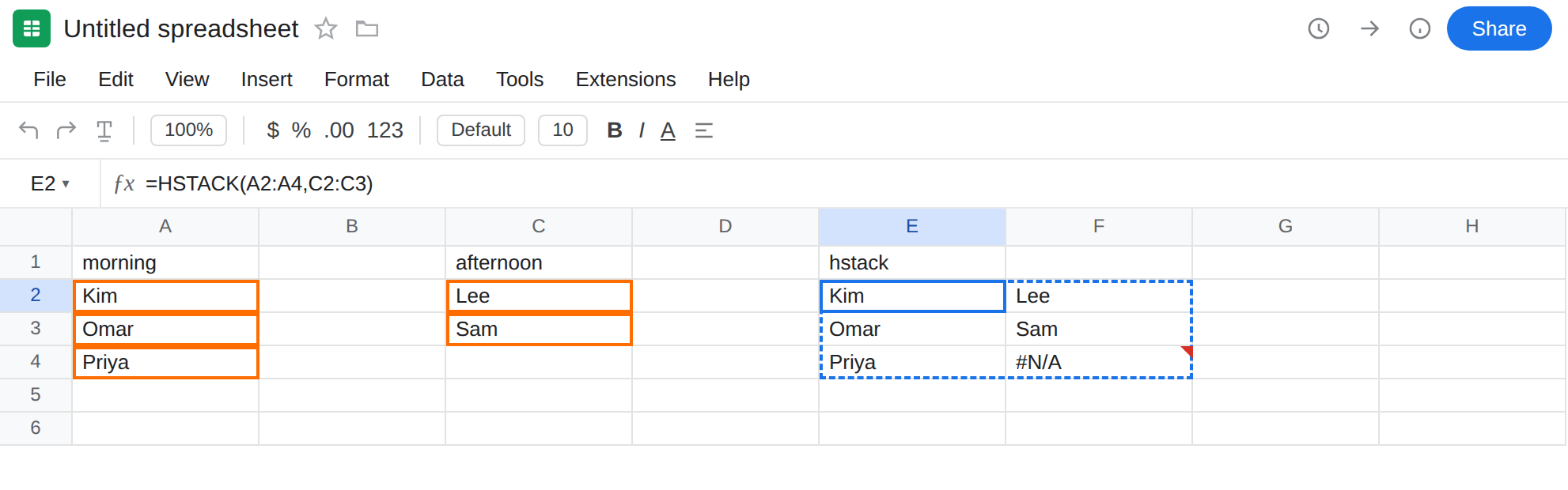
HSTACK pads the short column. In E1 type hstack. In E2 enter =HSTACK(A2:A4,C2:C3). The formula spills two columns and three rows. E2:E4 is Kim / Omar / Priya. F2:F3 is Lee / Sam. F4 is #N/A. There is no fourth afternoon name. HSTACK does not stop at two rows. It pads. Leave E2 as that spill so the #N/A stays visible.

VSTACK pads the narrow block. In A6 type role, B6 hours. A7 lead. B7 8. A8 dock. B8 6. A two-column block. In D6 type tag. D7 west. D8 east. One column. In E6 type vstack. In E7 enter =VSTACK(A7:B8,D7:D8). The spill is two rows of role/hours, then two more rows with west and east in the first column and #N/A in the second. Leave E7 broken-looking: those #N/A cells are the pad.

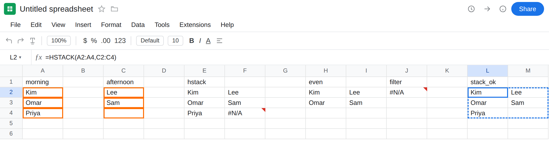
A control with matching sizes. In H1 type even. In H2 enter =HSTACK(A2:A3,C2:C3). Four cells, no #N/A. Two by two. That block is the control: equal height, no pad.

FILTER size is not this spill. In J1 type filter. In J2 enter =FILTER(A2:A4,C2:C5<>""). A2:A4 is three rows. C2:C5 is four. The cell errors (#N/A / #VALUE!). Tooltip: FILTER has mismatched range sizes. FILTER refuses the shapes. It does not pad. Leave J2 as the contrast. That page is FILTER range size.

What is actually wrong

• HSTACK of a 3-row array and a 2-row array is 3 rows tall. The missing two cells on the short side are #N/A. VSTACK of a 2-column array and a 1-column array is 2 columns wide. The missing column is #N/A.
• Those #N/A values are in the spill, often without the same “no match” tooltip you get from VLOOKUP. The formula ran. The arrays were different sizes. Padding is the contract.
• Empty cells in the source are not the same as a shorter range. HSTACK(A2:A4,C2:C4) with C4 blank spills a blank F4, not #N/A, because the ranges are the same height. C2:C3 is the short range that pads.
• FILTER with mismatched heights does not pad. It errors before it filters. J2 is that refusal. Do not read F4’s #N/A and J2’s #N/A as one bug.

This is not FILTER has mismatched range sizes. See FILTER range size. Equalize FILTER ranges. Do not HSTACK them to “make the heights match.”

This is not zero matching rows in FILTER. See FILTER no match. F4 is not “Lee was missing from a criteria.” Lee is in F2.

This is not a VLOOKUP miss and not QUERY empty output. See what #N/A means and QUERY no rows. No key was searched.

This is not a SEQUENCE / UNIQUE spill #REF!. Occupied cells would block HSTACK from writing at all. See SEQUENCE spill. If E2 is #REF! with Array result was not expanded, clear F4 or move the formula — that is occupancy, then you may still see pad #N/A after it spills.

Fix

Leave E2 and E7 as the padded spills. Leave J2 as the FILTER contrast. Leave H2 as the even control.

Give HSTACK the same height. In L1 type stack_ok. In L2 enter =HSTACK(A2:A4,C2:C4). F-side equivalent: afternoon in C2:C4 (C4 blank). The third afternoon cell is empty, not #N/A. If there is no third person, that blank is honest. If you meant only two rows of output, stack A2:A3 with C2:C3 (already H2).

Replace pad #N/A when a blank should print. In L6 enter =IFNA(HSTACK(A2:A4,C2:C3),""). F4-looking cell becomes empty. Use this when dashboards should not show #N/A for “no afternoon slot.” Do not use IFERROR — that would also hide a #REF! spill block. See IFERROR vs IFNA.

Trim instead of pad. =HSTACK(A2:A3,C2:C3) keeps the overlapping window. CHOOSEROWS / CHOOSECOLS on each piece before stacking does the same with an explicit row count.

VSTACK: same width. Put the tag in a two-column block (tag / blank hours) and stack that under A7:B8. Inside { }, watch array literal locale for ; vs ,.

If HSTACK / VSTACK shows #N/A in a corner of the spill, count rows and columns. Unequal sides pad. A FILTER tooltip with Expected row count is the other page.

This is not FILTER range size

FILTER walks a condition in lockstep with the data. Three data rows next to four condition rows is a refusal. Tooltip: FILTER has mismatched range sizes. The cell does not spill a padded table. See FILTER range size.

HSTACK and VSTACK are builders. They accept uneven pieces and fill the gap with #N/A. If Kim / Omar / Priya landed and only the last afternoon cell is #N/A, you stacked, you did not filter. Match heights, IFNA the pad, or shorten the tall side.