Fix HLOOKUP #N/A and #REF! in Google Sheets (no match vs row index)

HLOOKUP searches across the first row. The third argument is a row index, not a column index. #N/A is a miss in that first row. #REF! is an index taller than the range. Same error values as VLOOKUP. Different axis.

This page is HLOOKUP. Number vs text and a trailing space are the same key bugs as VLOOKUP no match. Do not redo those two recreates here.

Recreate it on a blank sheet

1. Open a blank spreadsheet. In A1 type sku, B1 101, C1 102. A2 name, B2 Widget, C2 Gadget. A3 price, B3 9.5, C3 12. E1 lookup, F1 hlookup.
2. In E2 type 999. In F2 enter =HLOOKUP(E2,B1:C3,2,FALSE). The cell shows #N/A. The tooltip is Did not find value ‘999’ in HLOOKUP evaluation.

F2 selected. Formula bar shows =HLOOKUP(E2,B1,2,FALSE). F2 is #N/A. Tooltip: Did not find value '999' in HLOOKUP evaluation. E2 is 999. B1 is 101. C1 is 102.

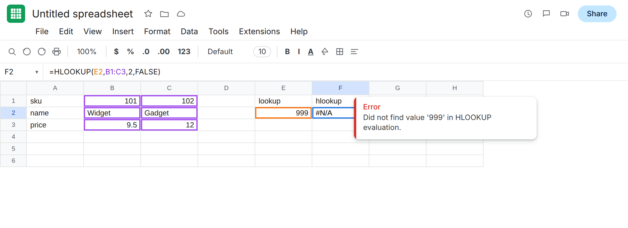
Leave F2 as the broken miss.

Second recreate — row index past the range. In E3 type 101. In F3 enter =HLOOKUP(E3,B1:C2,3,FALSE). Range B1:C2 is two rows. Index 3 asks for a third. The cell shows #REF!. The tooltip is HLOOKUP evaluates to an out of bounds range.

F3 selected. Formula bar shows =HLOOKUP(E3,B1,3,FALSE). F3 is #REF!. Tooltip: HLOOKUP evaluates to an out of bounds range. E3 is 101. F2 is still #N/A.

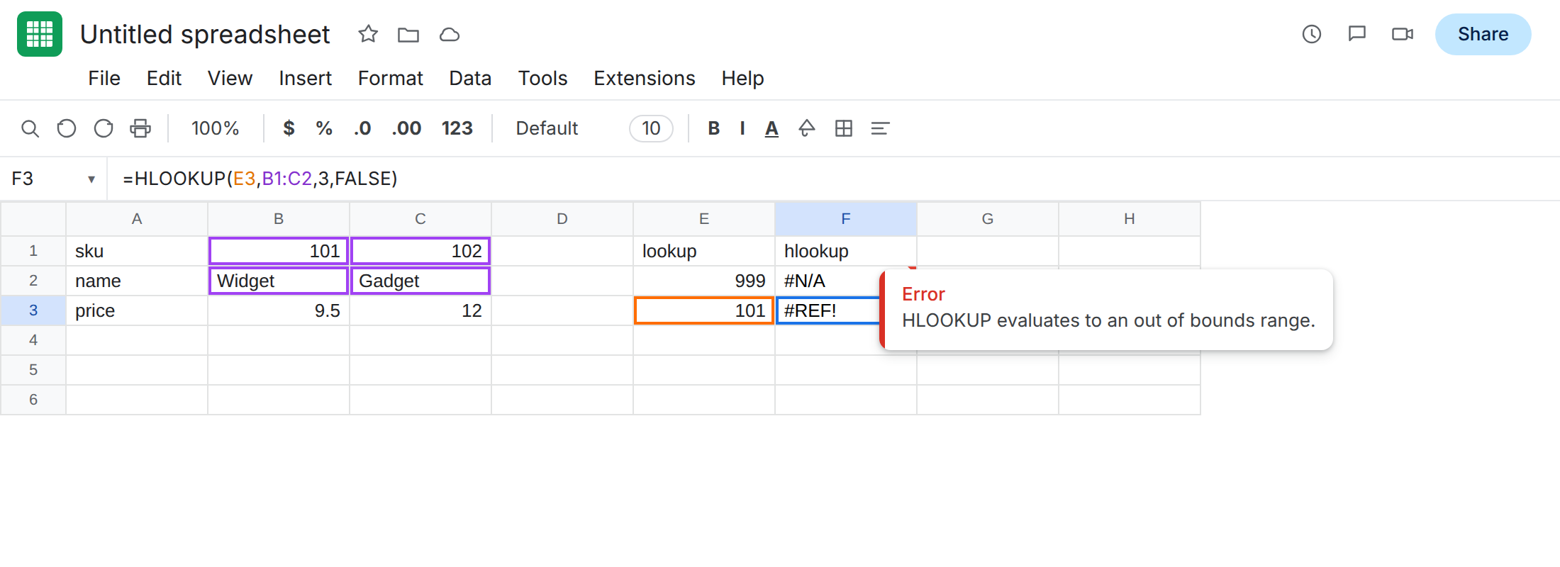
Leave F3 as the broken index.

What is actually wrong

• HLOOKUP always searches the first row of the range you give it. 999 is not in B1:C1. That is #N/A. Same idea as VLOOKUP missing a key in the first column. See what #N/A means.
• Range B1:C2 is two rows high. Index 3 is a third row that range does not contain. Row 3 is on the sheet (price), but it is outside the range you passed. HLOOKUP will not walk into it.
• VLOOKUP’s third argument counts columns. HLOOKUP’s third argument counts rows. =VLOOKUP(D2,A2:B2,3,FALSE) is VLOOKUP bad index. Same #REF! value. You are counting the wrong direction.
• A key you can see can still miss. Number vs text (101 vs '101) and a trailing space are still #N/A with FALSE. Those two cases live on VLOOKUP no match. HLOOKUP does not coerce them either.

This is not a deleted reference. The formula bar still shows HLOOKUP and a real range. See after you delete.

This is not a SORT or UNIQUE spill hitting a blocked cell. That #REF! tooltip is Array result was not expanded. See SORT / UNIQUE spill.

Fix

Leave F2 and F3 broken so both errors stay on the sheet.

Confirm the miss. In E2 type 101. F2 becomes Widget. Put 999 back. If changing the lookup value makes #N/A come and go, the function is working and the key is not in the first row.

When no match is a valid result. Then wrap only #N/A. In G1 type ifna. In G2 enter =IFNA(HLOOKUP(E2,B1:C3,2,FALSE),"none"). The cell shows none. Do not wrap F3 in IFNA. IFNA does not catch #REF!. See IFERROR vs IFNA.

Row index too big. Want the name from a two-row range: change the index to 2. In G3 enter =HLOOKUP(E3,B1:C2,2,FALSE). The cell shows Widget. Want the price: keep index 3 and extend the range down. In H3 enter =HLOOKUP(E3,B1:C3,3,FALSE). The cell shows 9.5.

H3 selected. Formula bar shows =HLOOKUP(E3,B1,3,FALSE). H3 is 9.5. G3 is Widget. G2 is none. F2 is still #N/A. F3 is still #REF!.

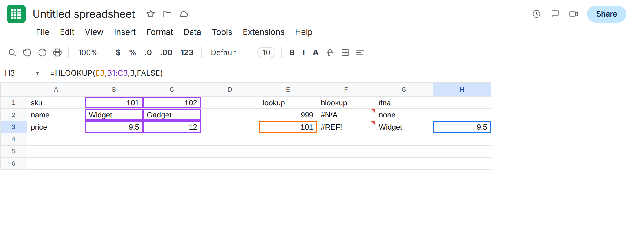
Count the rows in the range before you pick the index. Index 1 is the lookup row. Index 3 needs a range at least three rows tall.

If the sku is on the sheet and F2 is still #N/A, check type and LEN on the VLOOKUP page. IFNA will not.