A conditional formatting custom formula paints only the first column of a wide range

A conditional formatting custom formula is written for the top-left cell of the apply-to range. Sheets fills it across and down, the way a fill handle does. If the range is A2:C6 and the formula is =A2="open", column A tests column A. Column B tests column B, because the reference was relative and the fill moved it. The status word lives in column A. Column B is a person’s name. The name is not open, so only column A lights up. The rule looks like it ignored the rest of the range. The range is fine. The formula walked off the column you meant to test.

Locking both the row and the column, so every row copies row 2, is conditional formatting $. Text contains is not a formula. A caret in that rule is text contains. Keep the Google Sheets UI in English. Sheet Error is an independent formula-error library, not a Google product.

Recreate it on a blank sheet

1. Open a blank spreadsheet. In A1 type status, B1 owner, C1 hours. A2 open, B2 Ada, C2 5. A3 shut, B3 Bo, C3 2. A4 open, B4 Cy, C4 9. A5 open, B5 Di, C5 1.

Select the whole block. Select A2:C5. Format → Conditional formatting. The apply-to range reads A2:C5. If it reads A2:A5, you selected one column. Widen it before you judge the formula. Format rules: Custom formula is. Do not pick Text is exactly.

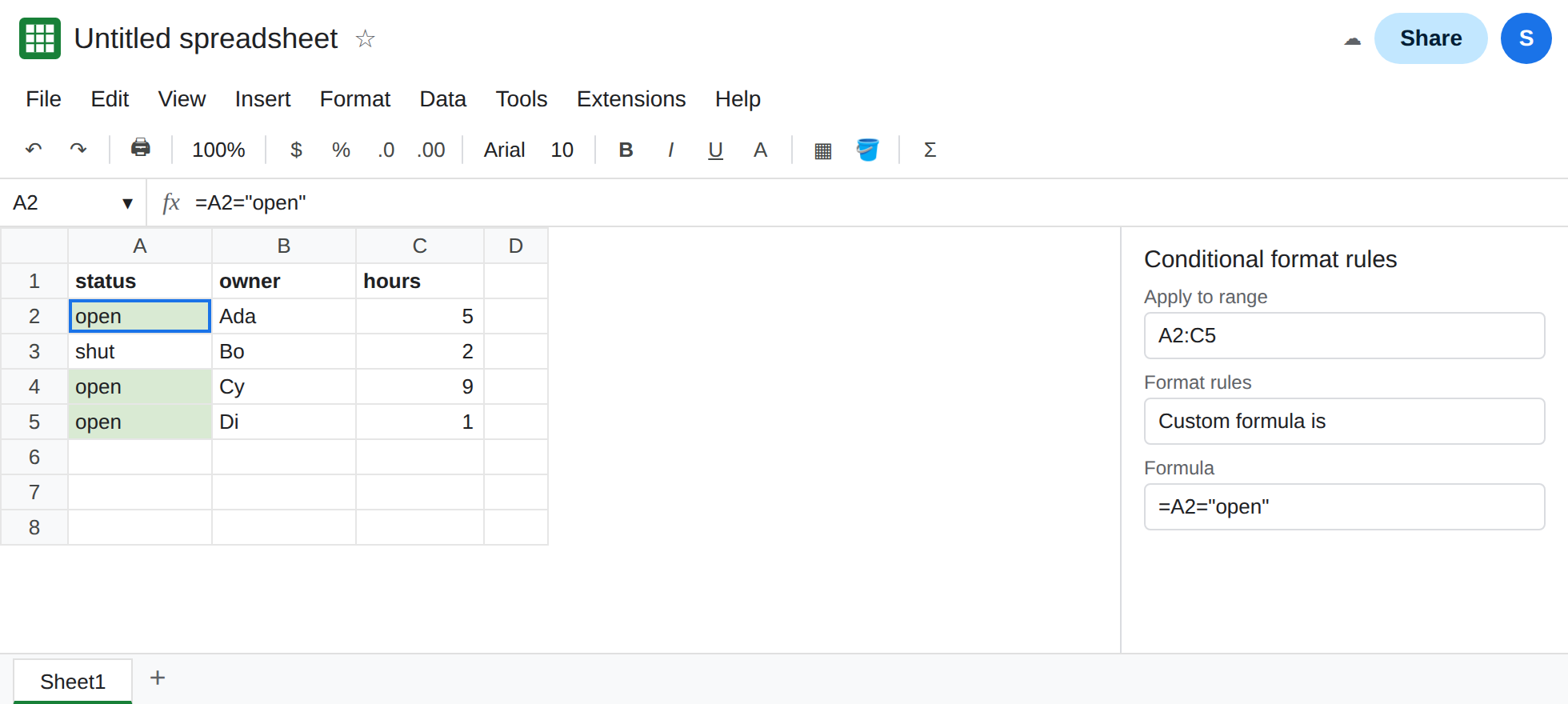
A relative formula paints one column. In the formula box enter =A2="open". Pick a fill color. Click Done. A2, A4, and A5 are filled. B2:C5 are not, including B2 next to a status of open. The apply-to range still says A2:C5. The rule ran on every cell. On B2 the filled formula is =B2="open", and Ada is not open. Leave this rule in place.

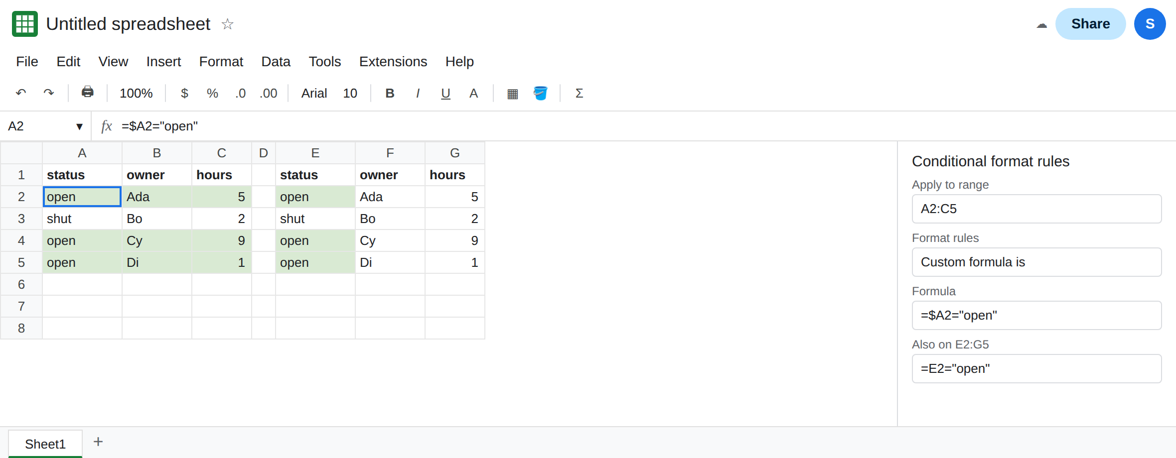
Lock the column. Edit the rule. Change the formula to =$A2="open". Done. Each open row fills across A:C. The shut row does not. $A keeps the test on status while the fill moves through owner and hours. The row number stays relative, so row 4 tests A4, not A2. Leave this as the working rule on A2:C5.

A formula that is itself a range does not spill paint. Add a second rule, or edit a copy of the block at E2:G5 with the same values. Custom formula =A2:C2="open", apply to E2:G5, will not paint three TRUE/FALSE cells the way ARRAYFORMULA spills. Conditional formatting wants one condition for the top-left cell. A range inside the formula is the wrong shape. You get a first-cell result, no fill, or a fill that does not follow the open rows. The working shape is =$A2="open", one test. Do not wrap it in ARRAYFORMULA. The format engine already fills.

The opposite bug, in one line. =$A$2="open" on a range that starts at row 2 paints every row whenever A2 is open, including the shut row. That is conditional formatting $. This page is the formula that paints too little. That page is the formula that paints too much.

There is no error triangle. A false test is no fill, not #N/A.

What is actually wrong

• One formula is stored, for the top-left cell of the apply-to range. Here that cell is A2. Filling to B2 changes A2 into B2 unless the column is locked. The apply-to box can list three columns while the paint stays in the first. Both facts are true at once.
• $ is per letter and per number. $A2 locks the column and lets the row move. That is the lock for “the whole row, based on column A.” A$2 locks the row and lets the column move, which paints a stripe of row 2’s test across the columns. $A$2 locks both.
• The first row of the range and the row number in the formula have to be the same row. If the apply-to range is A2:C5 and you write =$A5="open", row 2 of the sheet tests A5. You will paint the wrong rows and then widen the range again. Put the top-left row number in the formula.
• Two rules on the same range stack. A later rule does not prove the first formula was a range-size bug. Open the rule and read the formula before you add another color.
• Text must match. open with a trailing space fails =$A2="open" on that row only, which looks like a broken fill in the middle of the column. See CHAR(160) blanks.

A spilled FILTER of the open rows is a formula, not a paint rule. See FILTER no match.

Fix

Copy A2:C5 to E2:G5 and put =E2="open" on E2:G5 so the first-column-only paint remains on the sheet. On A2:C5 use the locked column.

Lock the column you are testing. Apply to A2:C5. Formula =$A2="open". Open rows fill from column A through column C. The shut row stays bare.

Apply to one column when the row fill is not what you want. Range A2:A5 and formula =A2="open" paints status only. You do not need $ until the range grows to the right. Add $A in the same edit that widens the range.

Prove the formula in a normal cell first. In I2 enter =$A2="open" and fill it down through I5. I2 TRUE, I3 FALSE, I4 TRUE, I5 TRUE. Paste that formula into the rule. If I2 is already wrong, the rule will be wrong. Do not put IFERROR around the custom formula. A false test should be unpainted.

If the apply-to range lists several columns and only the first is colored, the column letter in the formula is relative. Add $ in front of that letter. If every row is colored, including the rows that should fail, a $ is locking the row number. That is the other page.