

Fix SPARKLINE errors in Google Sheets (empty range or wrong argument)
Updated
SPARKLINE draws a tiny chart inside a cell from a numeric range and an optional list of options. An empty range, or an option Sheets does not know, is an error — often #N/A — not a blank sparkline you can ignore. The function is fine. The data or the option table is not.
This page is SPARKLINE. It is not IMAGE failed to load (a URL, a bitmap). It is not GOOGLEFINANCE #N/A (a ticker). A sparkline is not a finance quote and not an IMAGE fetch.
Recreate it on a blank sheet
Section titled “Recreate it on a blank sheet”- Open a blank spreadsheet. In A1 type
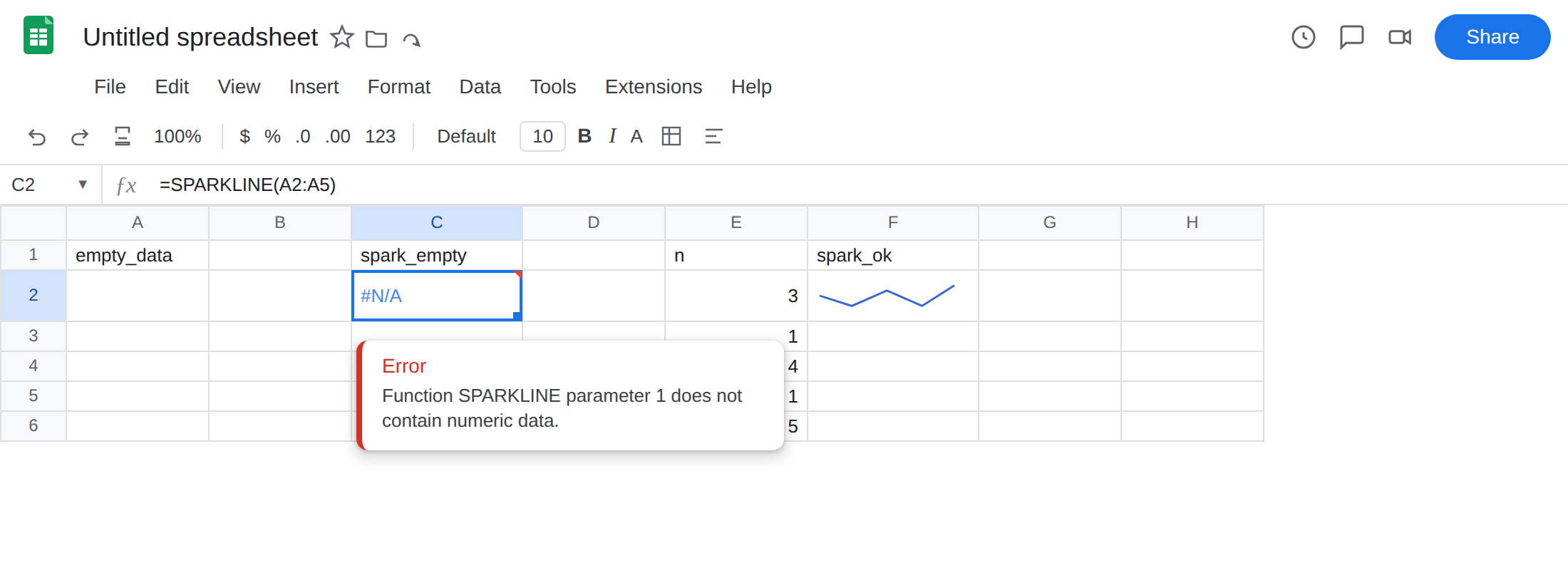
empty_data. Leave A2:A5 blank on purpose. - Empty range. In C1 type
spark_empty. In C2 enter=SPARKLINE(A2:A5). The cell shows#N/A(or a sparkline error for empty data). There are no numbers to plot. Leave C2 broken.
- A working mini chart in the next cell. In E1 type
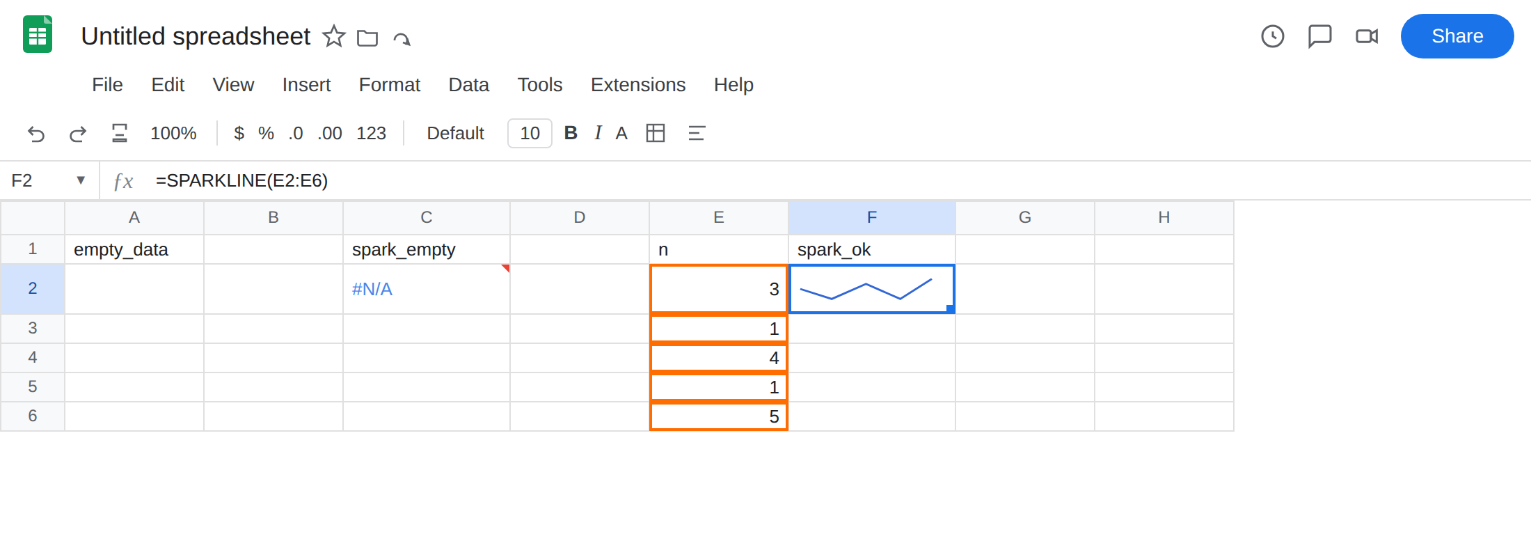
n. E23. E31. E44. E51. E65. In F1 typespark_ok. In F2 enter=SPARKLINE(E2:E6). F2 shows a small line chart. That cell is the control: same function, numeric data. Keep F2 working while you break the others.
- A bad option. In H1 type
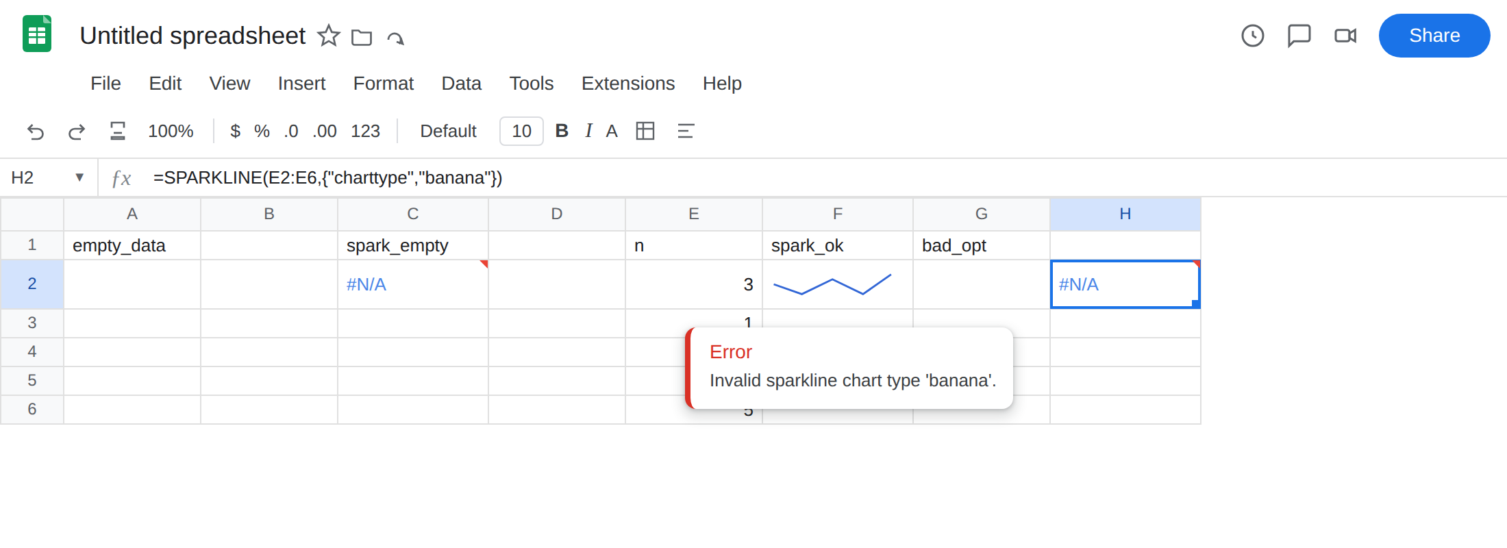
bad_opt. In H2 enter=SPARKLINE(E2:E6,{"charttype","banana"}). The cell errors (#N/A/ unknown chart type).bananais not a sparkline type. Valid types includeline(default),bar,column,winloss. Leave H2 broken.
- A good option on the same numbers. In H4 enter
=SPARKLINE(E2:E6,{"charttype","column"}). H4 shows a tiny column chart of 3, 1, 4, 1, 5. If{ }is#ERROR!with a Formula parse error, this spreadsheet’s locale uses\as the array column separator. Write{"charttype"\"column"}. See array literal locale. That parse error is not a sparkline miss.
Leave C2 and H2 as the broken formulas. Leave F2 (and H4) as working charts.
What is actually wrong
Section titled “What is actually wrong”SPARKLINEneeds numbers. A2:A5 is empty. Empty is not zero. The function has nothing to scale.#N/A(empty / no data) is that miss. Filling A2:A5 with0would chart a flat line — different from blank.- The second argument is a two-column map of option names to values. Unknown
charttype, a misspelled"colorr", or a one-column array that is not a pair, is a bad argument. H2 is that case. F2 omitted the argument and used the default line. - Text in the data range is skipped or poisons the chart depending on the mix. A range of
pcsis not a sparkline. Put numbers in E, labels in a header. SPARKLINEreturns one cell. It does not spill. A#REF!in F2 would mean something else overwrote the cell or the formula was deleted into#REF!. This recreate is#N/A/ invalid option, not a spill.
This is not IMAGE. IMAGE fetches a PNG/JPEG URL. A dead URL is failed to load. There is no charttype. See IMAGE failed to load. Putting a URL inside SPARKLINE will not paint a logo.
This is not GOOGLEFINANCE. A ticker miss is #N/A with no sparkline. You can chart values after Finance returns numbers (=SPARKLINE(GOOGLEFINANCE("CURRENCY:USDJPY","price",TODAY()-30,TODAY())) is a different, heavier formula). This page’s recreate does not call Finance. See GOOGLEFINANCE #N/A.
This is not a lookup miss. See what #N/A means. Do not wrap C2 in IFNA until you know you meant “no points.”
Leave C2 and H2 broken so the errors stay on the sheet.
Give it numbers. Keep F2: =SPARKLINE(E2:E6) is the working mini chart in the next cell. Point SPARKLINE at that numeric column, not at a blank A2:A5. If the source is a formula that can be empty, chart a helper that only contains numbers, or accept that a blank source is #N/A.
Use a documented option. Keep H4: =SPARKLINE(E2:E6,{"charttype","column"}). Other useful pairs: "color" / a color string, "linewidth" / a number for line, "xmin" "xmax" "ymin" "ymax" to lock scale. Do not invent "banana". Do not pass a single string as the second argument (SPARKLINE(E2:E6,"column") is the wrong shape — use the {option, value} array).
Empty vs zero. If you want a flat line for “no activity,” put 0 in the cells. If you want no chart until data exists, leave C2 as #N/A or wrap: =IF(COUNT(A2:A5)=0,"",SPARKLINE(A2:A5)). COUNT ignores blanks. IFERROR would also hide a bad charttype. Prefer COUNT for empty, and fix H2’s option by name.
Do not replace SPARKLINE with IMAGE of a chart screenshot. Do not call GOOGLEFINANCE to “fill” A2:A5 unless you actually want a quote series — and then handle Finance #N/A on that page first.
If SPARKLINE errors, ask whether the range has numbers and whether the option array uses a real charttype. F2 on this sheet is the picture of success: a mini chart in the cell next to 3, 1, 4, 1, 5.