Fix SUMIFS missing dates stored as text in Google Sheets

SUMIFS can return 0 when the invoice date is sitting on the sheet. There is no red triangle. The formula ran. It compared a real date serial to text that looks like a date. Those are not equal. The amounts next to the text dates never enter the total.

This page is date-as-text in SUMIFS / COUNTIFS. It is not CHAR(160) blanks (LEN is one too high and TRIM does not move). It is not CSV text vs number (sku 101 vs '101 after File → Import). It is not COUNTIFS range size (#VALUE! from different heights).

Recreate it on a blank sheet

1. Open a blank spreadsheet. File → Settings → Locale → United States so 3/4/2024 is 4 March, not 3 April. Display language English. In A1 type invoiced, B1 amount.
2. In A2 type an apostrophe then 3/4/2024. The cell is text, left-aligned. B2 40. In A3 type 3/4/2024 without an apostrophe so Sheets stores a real date. B3 15. In A4 type an apostrophe then 3/5/2024. B4 25. A2 and A4 look like dates. They are not.

SUMIFS against a real date. In D1 type as_of. In D2 enter =DATE(2024,3,4). In E1 type sumifs. In E2 enter =SUMIFS(B2:B4,A2:A4,D2). The cell shows 15. Only A3 matched. A2 looks like the same day and was skipped. Leave E2 as the broken total.

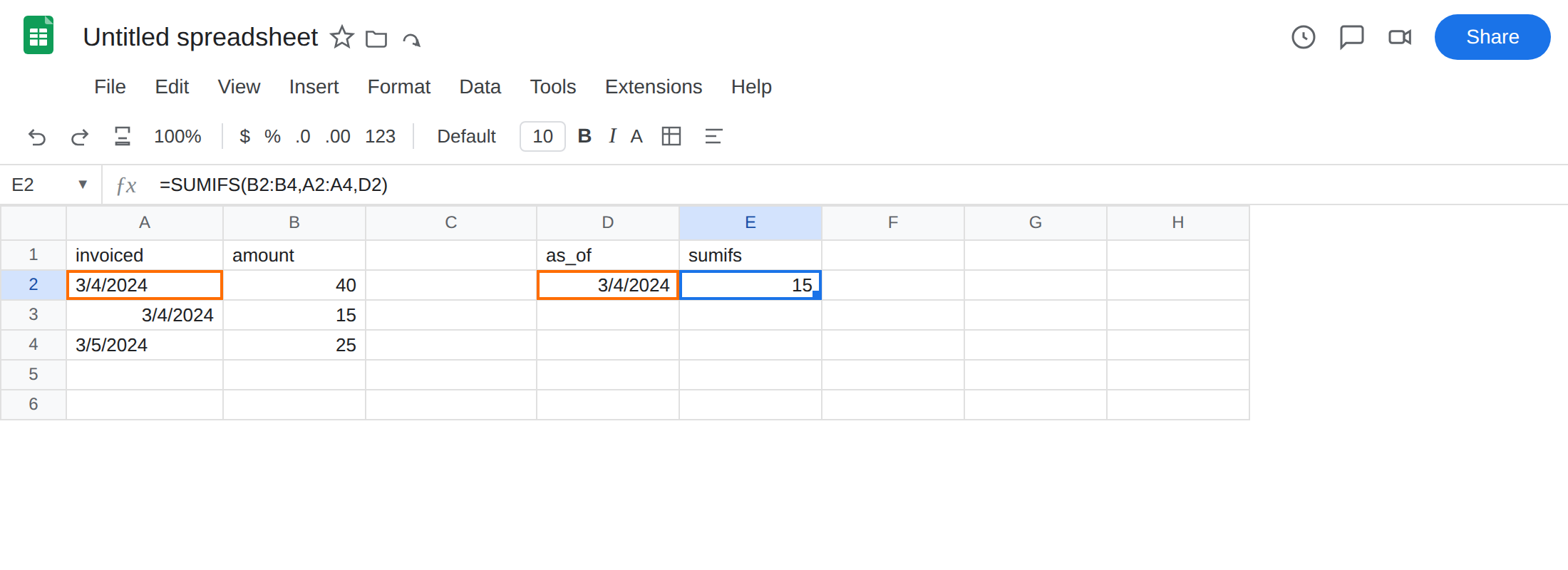
COUNTIFS on the same column. In E4 enter =COUNTIFS(A2:A4,D2). The cell shows 1. You can see two 3/4/2024 labels. The function counted one.

Date inequalities skip the text rows. In F4 enter =SUMIFS(B2:B4,A2:A4,">="&D2). A2 still misses. Confirm types: =ISNUMBER(A2) FALSE, =ISNUMBER(A3) TRUE. Same digits on the screen. Different types.

Leave E2 as the quiet 15.

What is actually wrong

• Sheets stores dates as numbers (serials). SUMIFS with D2 (DATE(2024,3,4)) compares that serial to each cell in A. A3 is a serial. A2 is the string 3/4/2024. They do not match. Amount 40 is ignored.
• File → Import, a CSV, or a paste from mail often leaves a date column as text. The column looks right. ISNUMBER is the check, not your eyes.
• A ">="&date criterion is a date compare. Text that looks like 3/4/2024 is not greater than a serial. It is a different value. The row drops out without #N/A.
• SUMIF (one criterion) has the same miss. This recreate uses SUMIFS because that is the form people copy into dashboards.

This is not CHAR(160). A2’s LEN is the length of the characters you typed. TRIM may not change it. There is no extra non-breaking space in this recreate. See CHAR(160) blanks when LEN is 4 on a three-digit sku and TRIM stays 4.

This is not sku text vs number after CSV import. See CSV text vs number. Ids do not become dates. Dates that stayed text are this page.

This is not #VALUE! from mismatched SUMIFS heights. See COUNTIFS range size. E2 is a number. This is not QUERY year(A) on TBD. See QUERY mixed dates.

Fix

Leave E2 as 15 so the miss stays visible.

Make a date helper, then sum that. In C1 type invoiced_date. In C2 enter =IF(ISNUMBER(A2),A2,IFERROR(DATEVALUE(A2),"")) and fill down through C4. C2 and C4 become real dates if the string matches this locale. C3 stays the serial it already was. In E6 enter =SUMIFS(B2:B4,C2:C4,D2). The cell shows 55 (40 + 15).

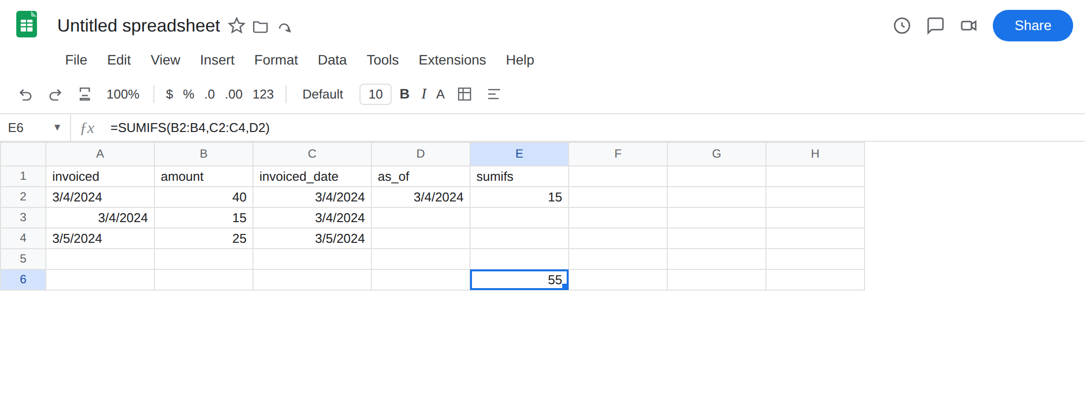
If DATEVALUE is #VALUE! on a helper row. The string is not a date in this locale (13/1/2024 on United States). That is DATEVALUE locale. Rewrite the text (3/4/2024 vs 4/3/2024) or use DATE(year,month,day) from split parts. Do not change Locale to rescue one import and break the rest of the file.

Convert the column once. Format A as Date only after the cells are serials. Format → Number → Date on text that still is text does not convert it. DATEVALUE (or split + DATE) does. Then point SUMIFS at the converted column.

Fix it at import when you still have the file. File → Import. Let Sheets convert dates, or parse them in a helper before any SUMIFS. Do not wrap E2 in IFERROR. There is no error to catch.

If SUMIFS of a date column is smaller than the rows you can see, test ISNUMBER on the date cells first. Text that looks like 3/4/2024 is this page.

Date serial vs looking like a date

A date you can read is not a date Sheets can compare. Left-aligned 3/4/2024, formula bar showing '3/4/2024, and ISNUMBER FALSE are the same story. Right-aligned date, formula bar showing 3/4/2024 without an apostrophe, ISNUMBER TRUE — that row will match DATE(2024,3,4) and ">="&D2.

SUMIFS will not “figure it out” because the characters look like a calendar. It does not run DATEVALUE for you. The CHAR(160) primer is leftover spaces. The CSV primer is leftover ids. This primer is leftover date text. Convert, then sum. Do not widen the criterion to "*3/4*" to catch the string — that abandons date math the next time you need a range of days.