TOCOL with scan_by_column TRUE reads down each column and reorders the list

TOCOL stacks a block into one column. The third argument, scan_by_column, chooses the walk. Omit it, or pass FALSE, and Sheets reads the first row left to right, then the next row. Pass TRUE and Sheets reads the first column top to bottom, then the next column. On a grid of 1 2 3 / 4 5 6, the default second value is 2. With TRUE, the second value is 4. Both spills are six numbers. Neither is an error. They are different orders.

Blanks and errors, and the ignore codes 0 through 3, are TOCOL ignore. A blocked spill is TOCOL / TOROW. Keep the Google Sheets UI in English. Sheet Error is an independent formula-error library, not a Google product.

Recreate it on a blank sheet

1. Open a blank spreadsheet. In A1 type 1, B1 2, C1 3. A2 4, B2 5, C2 6. Two rows, three columns. No blanks.

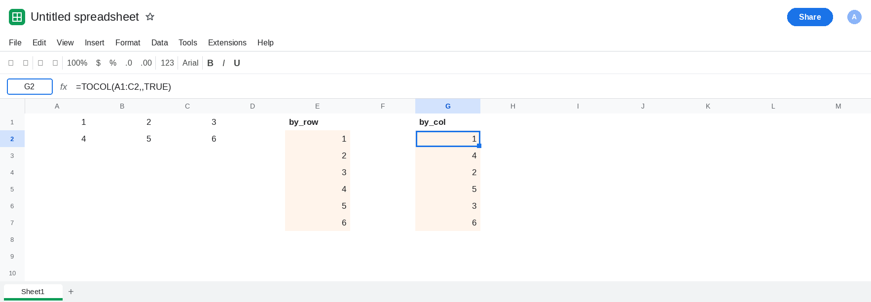
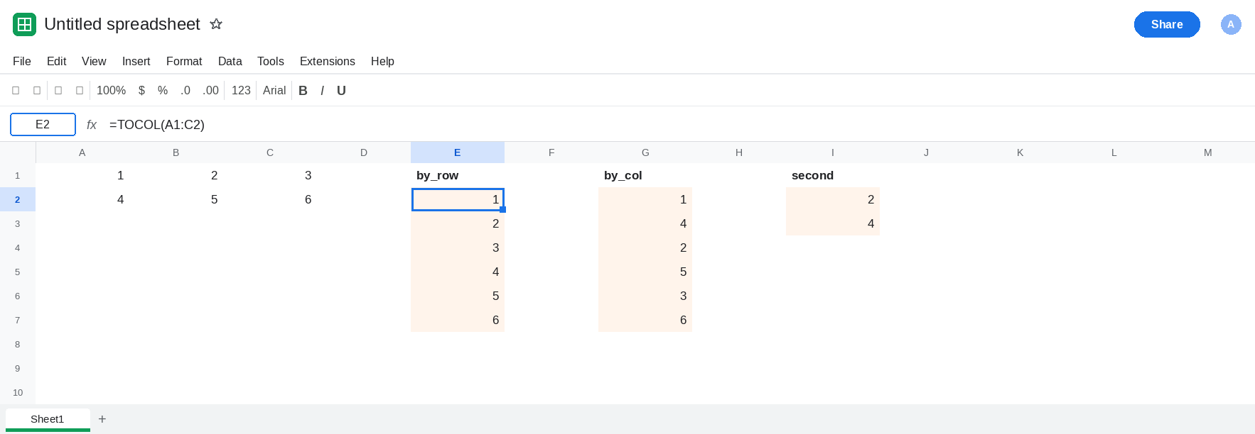
Row order, the default. Leave E2:E7 empty. In E1 type by_row. In E2 enter =TOCOL(A1:C2). The spill is 1, 2, 3, 4, 5, 6. Position 2 is 2, the rest of the first row, not the rest of the first column. That column is the control.

Column order. Leave G2:G7 empty. In G1 type by_col. In G2 enter =TOCOL(A1:C2,,TRUE). The blank second argument leaves ignore at its default, keep everything. TRUE is the scan. The spill is 1, 4, 2, 5, 3, 6. Position 2 is 4. Same six numbers. The pairs that were side by side are now two apart. Leave G2 as that order.

Position 2, so the reorder is a single cell. In I1 type second. In I2 enter =INDEX(TOCOL(A1:C2),2). I2 is 2. In I3 enter =INDEX(TOCOL(A1:C2,,TRUE),2). I3 is 4. A lookup that takes “the second item” changed because the scan changed. Leave I2 as 2 and I3 as 4.

TRUE is not an ignore code. In I5 enter =TOCOL(A1:C2,1). Ignore 1 drops blanks. This grid has no blanks, so I5:I10 matches E2:E7, the row order. The 1 did not walk by column. In I12 enter =TOCOL(A1:C2,1,TRUE). The order matches G2, because of TRUE, and the length is still six, because there was nothing to drop. People pass TRUE thinking the output is a column and the flag means “skip blanks.” The output is a column either way. Leave I3 as 4.

TOROW uses the same third argument and writes across. TRUE still means column-major. The spill direction stays a row. See TOROW width when that row cannot place itself. FLATTEN has no scan flag; it is always row by row. See FLATTEN vs TOCOL.

What is actually wrong

• Default TOCOL is row-major. scan_by_column TRUE is column-major. E2 and G2 are the demonstration. Nothing was sorted. 1 still comes first only because it is the top-left cell either way.
• The second argument is ignore, not direction. Leaving it blank in G2 is required so TRUE lands in the third slot. =TOCOL(A1:C2,TRUE) passes TRUE as ignore. TRUE coerces to 1, which means drop blanks, and the scan stays row-major. That call matches E2 on this grid. It is not G2.
• INDEX of position 2 is the first place a downstream formula notices. I2 versus I3. A VLOOKUP built on the stacked list will miss for the same reason: the keys moved.
• Ignore codes still apply on top of the scan. They remove cells. They do not reorder the ones they keep. The ignore page is TOCOL ignore. This grid was kept clear of blanks so the order is the only change.
• A value in E3 makes E2 #REF! because the spill cannot expand. G2 has the same rule, six cells down. That overwrite is TOCOL / TOROW. G2’s path is empty, which is why you see 4 instead of #REF!.

Fix

Leave G2 as the column-major spill if you wanted that order. Leave E2 as the row-major spill if you did not.

Pick the walk in the third argument. Keep E2 when the sheet is read like a sentence, across then down. Keep G2 when each column is a record that should stay together: 1 then 4, then the next column. In K2 enter =TOCOL(A1:C2,0,FALSE) if you want the default written out. It matches E2. 0 means keep blanks and errors. FALSE means row-major.

Do not pass TRUE in the ignore slot. If a stacked list lost its blanks and also looks row-major, the TRUE is argument two. Move it to argument three, and pass 0, 1, 2, or 3 for ignore on purpose.

Do not wrap G2 in SORT to “undo” a scan you did not intend. SORT will order the numbers 1 through 6 and destroy both layouts. Delete the third argument.

If the second value of a TOCOL is the cell under the first one, scan_by_column is TRUE. Omit it, or pass FALSE, for across-then-down. If blanks disappeared, you changed ignore, which is the other page. If the cell is #REF!, the column under the formula is occupied.