FILTER blank cells, empty strings, and spaces are not the same test

FILTER keeps rows whose condition is true. The condition A2:A="" is true for a cell you never typed in and for a formula that returns "". It is false for a space, for 0, and for text. The spill is a real list of amounts. It is not #N/A, and it is not “only the formula blanks.”

Sku 999 matching nothing is FILTER #N/A, tooltip No matches are found in FILTER evaluation. Do not use a missing sku as this recreate. If your blank test matches nothing, you will see that tooltip, and the cause is still the condition on this page.

Recreate it on a blank sheet

1. Open a blank spreadsheet. Keep the Google Sheets UI in English. In A1 type label, B1 amount.

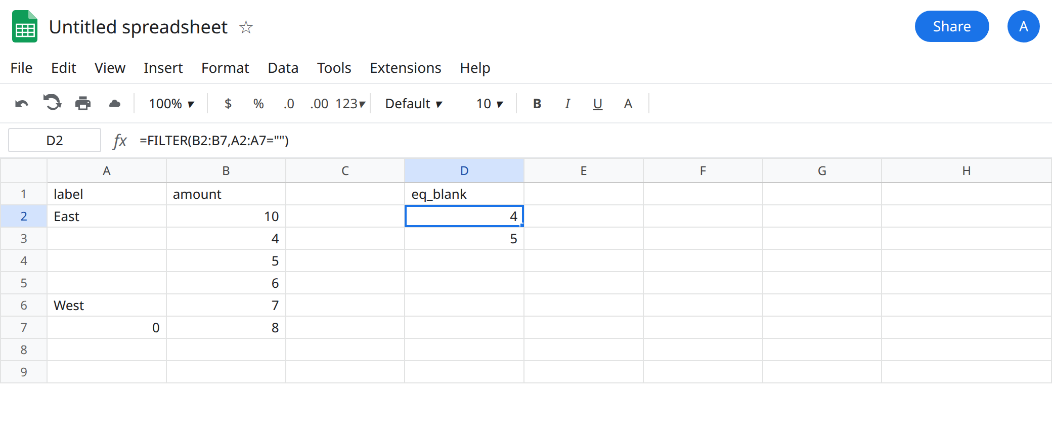
A2 East, B2 10. Leave A3 empty. B3 4. In A4 enter ="". B4 5. In A5 type one space. B5 6. A6 West, B6 7. In A7 type 0. B7 8. Do not type a space in A3. =ISBLANK(A3) is TRUE. =ISBLANK(A4) is FALSE. =LEN(A5) is 1.

Empty-string condition. In D1 type eq_blank. In D2 enter =FILTER(B2:B7,A2:A7=""). The spill is 4 and 5. B3 was truly blank in column A. B4 was a formula empty string. The space row (6), the zero (8), East, and West are out. The result is not #N/A. Two rows matched.

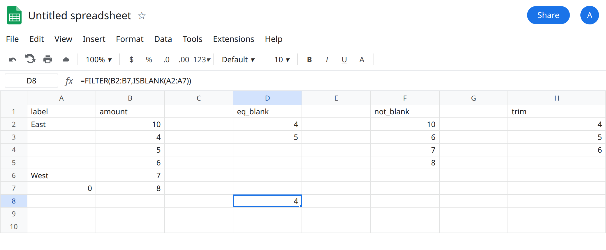
Not equal to empty string. In F1 type not_blank. In F2 enter =FILTER(B2:B7,A2:A7<>""). The spill includes 10, 6, 7, and 8. The space is still here. The zero is still here. 4 and 5 are gone. “Show me everything filled in” is false for a space: the cell is not empty, and it still looks empty on the screen if you do not check LEN.

Space-aware blank. In H1 type trim. In H2 enter =FILTER(B2:B7,LEN(TRIM(A2:A7))=0). The spill is 4, 5, and 6. TRIM turns a normal space into empty text, so the space row joins the blanks. It does not turn 0 into blank. 8 stays out. A non-breaking space is not always removed by TRIM. That character is CHAR(160) blanks.

Leave D2 as 4 and 5. If someone asked for “formula blanks only,” D2 is the wrong list because 4 is in it. If someone asked for “visually empty,” D2 is the wrong list because 6 is not in it.

What is actually wrong

• ="" in a FILTER condition is the same test as A3="" in one cell. In Google Sheets that comparison is TRUE for a never-used cell and TRUE for ="". ISBLANK vs empty disagrees: ISBLANK is FALSE on A4. FILTER does not call ISBLANK unless you write it.
• FILTER(..., ISBLANK(A2:A7)) keeps only A3’s amount 4. A4 drops out. People swap ="" and ISBLANK and think the function is unstable. The two tests are different. Write the one you measured.
• A space is not either of those blanks. F2 keeps it. D2 drops it. LEN is 1. Looking at the grid is not enough, because the space has no ink.
• 0 is a number. It fails ="". It fails ISBLANK. It stays in F2. Do not “clean zeros” with a blank filter.
• Several conditions are AND, and + is OR. That confusion is FILTER OR vs AND. This page uses one condition so the blank test is the only variable.
• Mismatched heights are a different #N/A: FILTER has mismatched range sizes. See FILTER range size. D2’s two ranges are both six rows.

If you change the labels until nothing matches, FILTER returns #N/A and the tooltip is No matches are found in FILTER evaluation. That display is FILTER #N/A. The repair is still the condition, not a fake sku.

Including the header by accident changes the test. =FILTER(A1:B7,A1:A7="") uses seven rows and the header text label, which is not blank, so the amounts can still spill, but the ranges must stay the same height. Dropping the header on only one side is the mismatched-size #N/A on FILTER range size. Keep D2 on A2:A7 so the blank test is the only thing you are reading. A blank amount next to a real label is a different column: =FILTER(A2:A7,B2:B7="") returns labels whose amount cell is empty, which is East’s neighbor only if you clear B2. Do not flip the columns and expect the spill of 4 and 5.

Fix

Leave D2 and F2 on the sheet. They are the two definitions.

Truly empty only. In D8 enter =FILTER(B2:B7,ISBLANK(A2:A7)). The spill is 4. A4’s formula blocks ISBLANK.

Blank or formula empty, not spaces. Keep D2.

Blank, formula empty, or ordinary spaces. Keep H2. If CHAR(160) is in the column, nest SUBSTITUTE or CLEAN the way the CHAR(160) page does, then test length. Do not switch to ="" and hope the special space counts as empty.

Do not wrap D2 in IFNA to drop the space row. D2 is not #N/A. IFNA does nothing to a spill of 4 and 5. IFERROR is the wrong wrapper if a later edit makes the ranges mismatch: you would hide the size error. See IFERROR vs IFNA.

If the spill has both the untouched cell and the ="" formula, you used ="". If the space amount is missing and you needed it, test LEN(TRIM(...))=0. If the cell is #N/A and the tooltip says no matches, the condition excluded every row, including the blanks you thought you had.