UNIQUE with by_col TRUE drops a duplicate column, so a day of numbers looks gone

UNIQUE(range, TRUE) compares columns. When two columns hold the same values from top to bottom, one of them is removed. The spill is shorter across, and a day of numbers looks deleted. Nothing errored. Default UNIQUE on the same block compares rows and keeps both columns, because no two rows are the same tuple.

The page that shows a header row mon, tue, wed, mon and the third argument exactly_once is UNIQUE by_col. Case and accents are UNIQUE case. Keep the Google Sheets UI in English. Sheet Error is an independent formula-error library, not a Google product.

Recreate it on a blank sheet

1. Open a blank spreadsheet. In A1 type mon, B1 tue, C1 wed. Those labels stay outside the formula. In A2 type 10, B2 10, C2 12. A3 20, B3 20, C3 15. A4 30, B4 30, C4 18. Monday and Tuesday are the same three numbers. Wednesday is not.

Rows, the control. Leave E2:G4 empty. In E1 type rows. In E2 enter =UNIQUE(A2:C4). The spill is three rows and three columns. 10 / 10 / 12, then 20 / 20 / 15, then 30 / 30 / 18. No two rows matched, so nothing dropped. Tuesday is still there. That block is what people expect from a “unique” of this table.

Columns. Leave E6:F8 empty. In E5 type by_col. In E6 enter =UNIQUE(A2:C4,TRUE). The spill is three rows and two columns: 10 / 12, 20 / 15, 30 / 18. The second 10, 20, 30 is gone. There is no error triangle. TRUE did not mean “be stricter about rows.” It changed the axis. Leave E6 as that narrower spill.

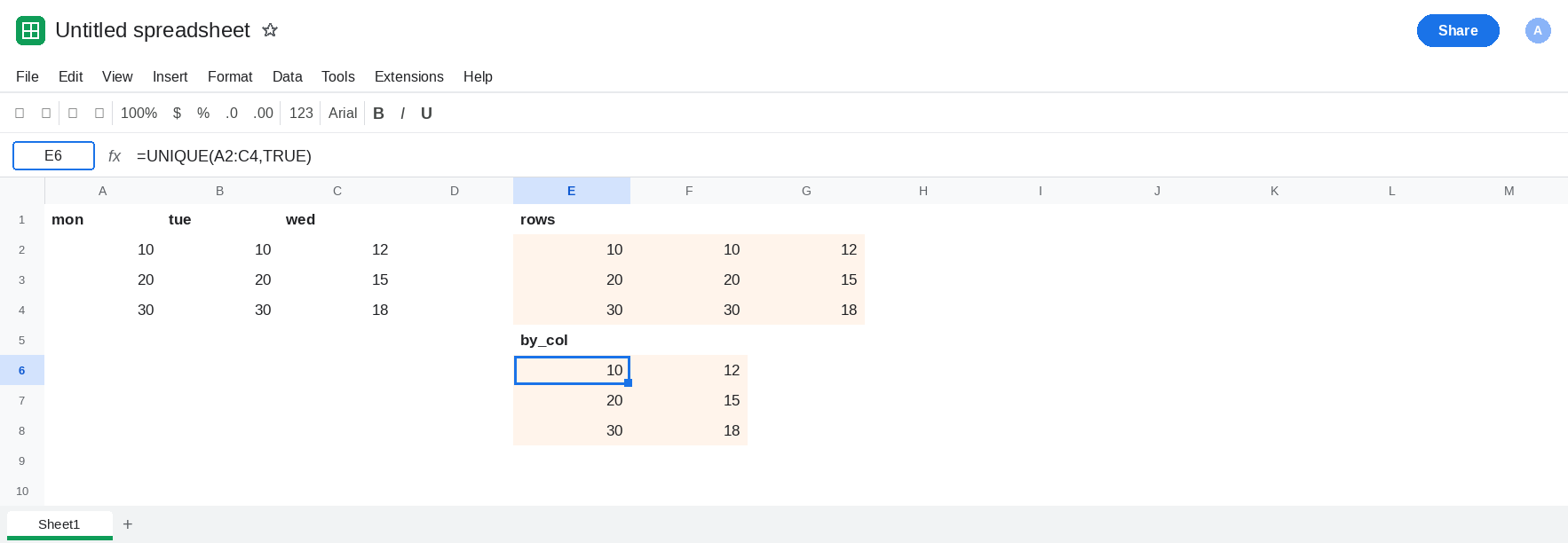
A repeated row is the other axis. In A5 type 10, B5 12, C5 15. In A6 type 10, B6 12, C6 15. Monday and Tuesday now differ in those two rows, so this block is no longer the E6 vanish. In E10 enter =UNIQUE(A2:C6). The second 10 / 12 / 15 drops. Five source rows become four. In E15 enter =UNIQUE(A2:C6,TRUE). You still get three columns, and both copies of 10 / 12 / 15 are still in the spill. TRUE did not remove the duplicated row. Row dedupe is E10. The vanished Tuesday is E6, which still points at A2:C4. Leave both.

Including A1:C1 in the range changes the test. mon and tue are different headers, so those columns are no longer identical even when A2:C4 matches B2:B4. The vanish on this page uses A2:C4 on purpose.

What is actually wrong

• The second argument is the axis. Omitted or FALSE means whole rows. TRUE means whole columns. E2 and E6 are the same numbers under those two rules.
• A column drops only when every cell matches the other column, in order. Monday 10, 20, 30 and Tuesday 10, 20, 30 are one column. Change B4 to 31 and Tuesday stays, because the columns differ in the last row.
• Headers count if they are inside the range. mon versus tue keeps both columns. That is why this recreate leaves row 1 out of UNIQUE.
• exactly_once is the third argument. =UNIQUE(A2:C4,FALSE,TRUE) would drop a row that appears twice. It does not explain a missing Tuesday. See UNIQUE by_col.
• A #REF! under the spill means a cell was already filled. E6 is a real two-column spill. See SORT / UNIQUE spill only when the tooltip says the array was not expanded.

Fix

Leave E6 as the two-column spill.

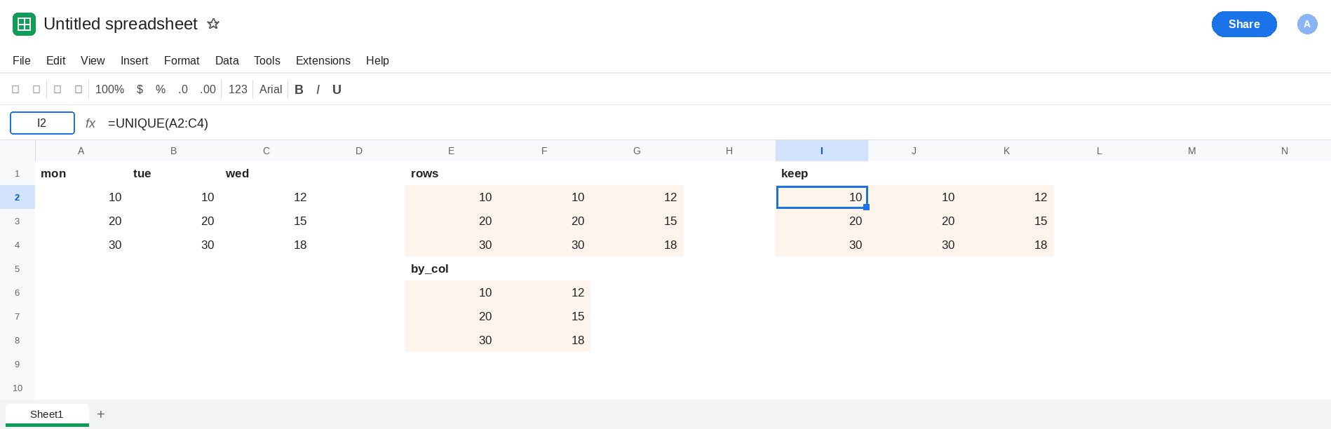
Dedupe rows by omitting the axis. In I1 type keep. In I2 enter =UNIQUE(A2:C4). I2 matches E2: three columns, Tuesday included. Use this when the table is a list of records and a copied day should remain until the rows themselves repeat.

Use TRUE only for a horizontal list. A row of labels such as mon, tue, wed, mon is the case UNIQUE by_col already builds. Point TRUE at that row. Do not point it at A2:C4 to “clean” a vertical log.

Do not wrap E6 in IFERROR. It is not an error. The missing column is the answer by_col is defined to give.

If a day disappeared and the formula’s second argument is TRUE, the columns matched and the axis is wrong for a row log. If a repeated sku vanished entirely, the third argument is TRUE and you are on the by_col primer. If the spill says it would overwrite a neighbor, the cells under the formula are occupied.