Fix TOCOL in Google Sheets when ignore 2 or 3 swallows errors or blanks

TOCOL(array, [ignore], [scan_by_column]) flattens a block into one column. ignore 0 keeps every cell. 1 drops blanks only. 2 drops errors only. 3 drops blanks and errors. The dangerous codes are 2 and 3: a #DIV/0!, #N/A, #VALUE!, or #REF! inside the source is removed from the result, so the stack looks clean while the source is still broken. scan_by_column TRUE changes the order of whatever survived. It does not change the ignore rule. Pointing it the wrong way looks like a different filter.

This page is ignore 2 and 3, and the scan flag. The blocked spill and the first look at ignore 1 are TOCOL / TOROW. FLATTEN, which cannot ignore, is FLATTEN vs TOCOL. Keep the Google Sheets UI in English.

Recreate it on a blank sheet

1. Open a blank spreadsheet. In A1 type am, B1 mid. A2 Kim. Leave B2 empty. In A3 enter =1/0. B3 Omar. A3 shows #DIV/0!. One blank, one real error, two names.

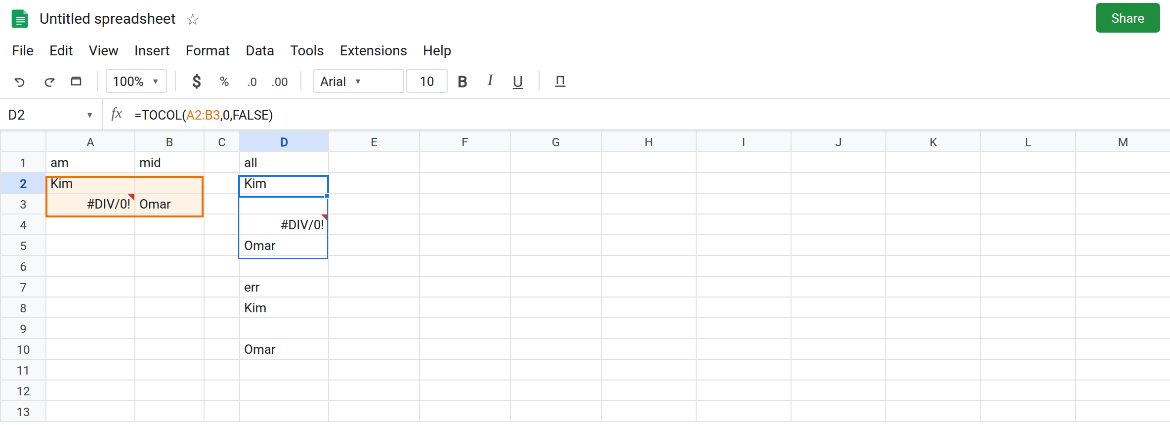
Ignore 0, everything. In D1 type all. Leave D2:D5 empty. In D2 enter =TOCOL(A2:B3,0,FALSE). The spill is Kim, blank, #DIV/0!, Omar. Row by row. The error is visible in the stack. That column is the control: you can still see the bug.

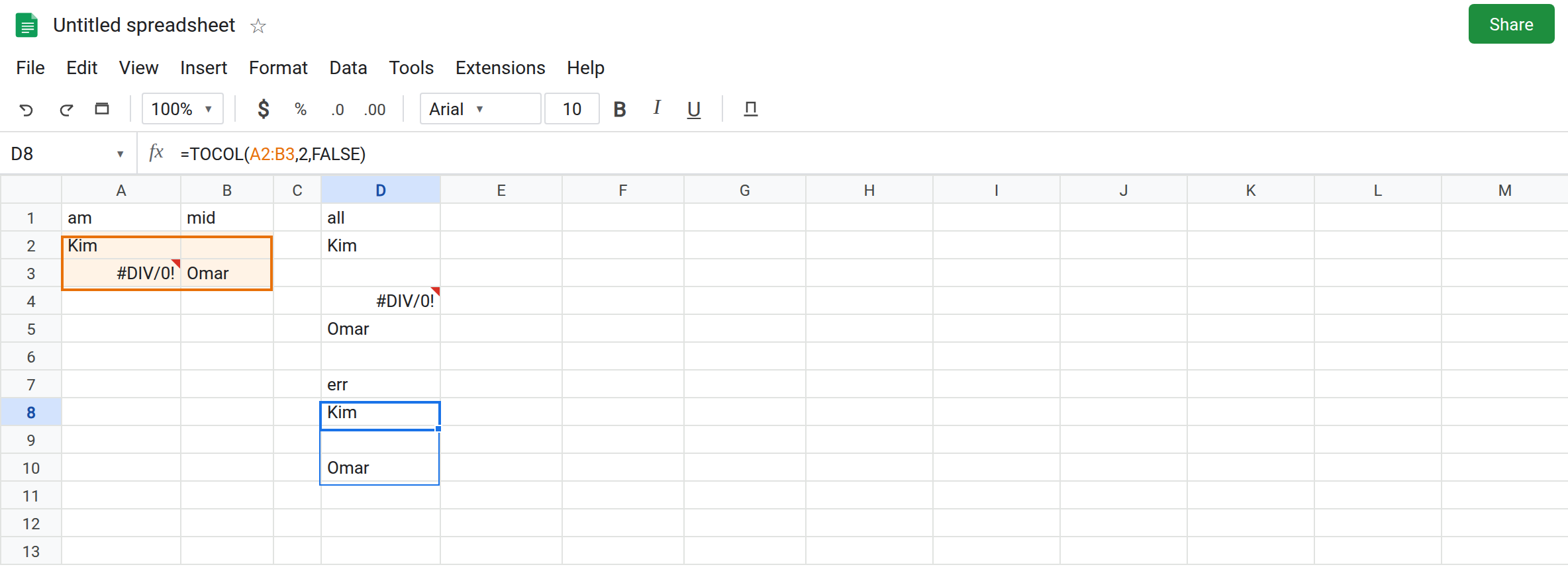
Ignore 2 drops the error and keeps the blank. In D7 type err. Leave D8:D11 empty. In D8 enter =TOCOL(A2:B3,2,FALSE). The spill is Kim, blank, Omar. A3’s #DIV/0! is gone. B2’s blank remains as an empty spilled cell. The stack is one row shorter and looks “fixed.” A3 is still #DIV/0! on the sheet. Leave D8 as that quiet column.

Ignore 3 drops both. In F1 type both. In F2 enter =TOCOL(A2:B3,3,FALSE). The spill is Kim, Omar only. The blank and the #DIV/0! are both gone. Two names, no hint that A3 is broken. Leave F2 as that pair.

Ignore 1 is the opposite hole. In F5 enter =TOCOL(A2:B3,1,FALSE). Blanks go, errors stay. The spill is Kim, #DIV/0!, Omar. If you wanted names only, F5 still shows the error. If you wanted to notice the error, F5 is the one that does. F2 does not.

Scan by column, same ignore. In H1 type down. In H2 enter =TOCOL(A2:B3,0,TRUE). Ignore 0, scan by column. The spill is Kim, #DIV/0!, blank, Omar. Same four values as D2, different order. In H7 enter =TOCOL(A2:B3,2,TRUE). Ignore 2 still drops A3. The order of what remains is column-wise: Kim, blank, Omar — on this tiny grid that can look identical to D8. Widen the block if you need to see the order change. The point is the flag did not restore #DIV/0!. Leave H2 as the reordered full stack.

Leave D8 and F2 as the stacks that hide A3. Leave A3 as #DIV/0!.

What is actually wrong

• Ignore 2 means “skip cells that are errors.” It does not fix the cell. A3 still divides by zero. Downstream formulas that read D8 never see it, so a later total can be “right” in the stack and wrong in the source.
• Ignore 3 is 1 and 2 together. A short list of names is not evidence that the block was clean. F2.
• Ignore 1 will not hide #DIV/0!. If the error is still in the stack, you did not use 2 or 3. You used 0 or 1.
• scan_by_column is order only. FALSE or omitted walks each row left to right, then the next row. TRUE walks each column top to bottom, then the next column. People pass TRUE because the output is a column and assume that also means “skip blanks.” It does not.
• TOROW uses the same ignore codes and spills sideways. Hiding an error in a header row is the same bug on the other axis. See TOROW spill when the failure is width, not a missing #DIV/0!.
• A blocked spill is still #REF! and still shows the error in the tooltip as an occupied cell. Ignore 2 does not turn that #REF! into a short list. The formula never returned. See TOCOL / TOROW.

This is not IFERROR around the source. See IFERROR hides the cause. Ignore 2 is a filter. IFERROR is a replacement. Both can make A3’s bug invisible. They are different formulas.

Fix

Leave D8 and F2 as the hiding stacks. Leave A3 broken so the source error stays visible.

Stack first, decide second. Keep D2 while you repair A3. When A3 is a real number, D2’s third spilled cell becomes that number.

Drop blanks only. =TOCOL(A2:B3,1,FALSE) after A3 is fixed, if the blank in B2 should not become a row. Until A3 is fixed, ignore 1 keeps the error in the stack on purpose.

Names only, after the errors are gone. Ignore 3 is reasonable on a block you have already checked, or on text columns that cannot contain a formula error. It is a poor default on a block that still has =1/0.

Order. Pass TRUE only when the source is stored in columns (a week down each column) and the stack should read that way. Leave it FALSE when the source is a row-wise table.

Do not wrap D2 in IFERROR. You would hide both a blocked spill and the #DIV/0! you just made visible. See IFERROR vs IFNA.

If the stack is missing a cell that shows #DIV/0! or #N/A in the source, ignore is 2 or 3. If the order is column-wise, the third argument is TRUE. If the tooltip names a cell under the formula, ignore is not the bug.