LOOKUP with one array is always approximate, and the shape picks the axis

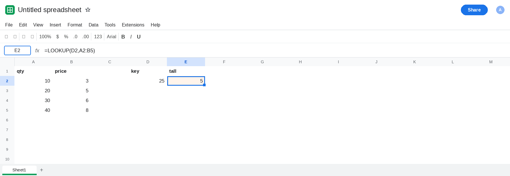
LOOKUP(key, array) is the array form. There is no fourth argument and no FALSE. The search is approximate, and the range is supposed to be sorted ascending along the axis Sheets picks from the shape. More rows than columns: search the first column, return the last column. More columns than rows: search the first row, return the last row. A qty of 25 on breaks 10, 20, 30, 40 returns the price beside 20. It does not return #N/A.

The three-argument call, with a separate result vector, is LOOKUP approximate. This page is the one-range form and the wide-versus-tall switch. Keep the Google Sheets UI in English. Sheet Error is an independent formula-error library, not a Google product.

Recreate it on a blank sheet

1. Open a blank spreadsheet. In A1 type qty, B1 price. A2 10, B2 3. A3 20, B3 5. A4 30, B4 6. A5 40, B5 8. The qty column ascends. A2:B5 is taller than it is wide.

Tall array. In D1 type key. D2 25. In E1 type tall. In E2 enter =LOOKUP(D2,A2:B5). E2 is 5. The largest qty that is still <= 25 is 20, and 20 sits beside price 5. There is no triangle. Nothing in the formula says approximate. Leave E2 as 5.

The ends. In E4 enter =LOOKUP(5,A2:B5). E4 is #N/A. 5 is smaller than every qty, so there is no break less than or equal to the key. That is the one missing-key case this function reports. In E5 enter =LOOKUP(100,A2:B5). E5 is 8. 100 is past the last break, so the last row wins. Leave E4 as #N/A and E5 as 8.

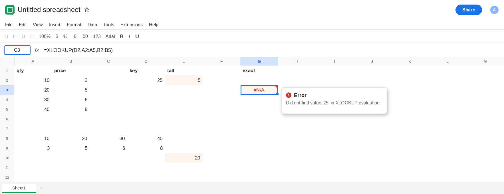
Wide array, same breaks. In A8 type 10, B8 20, C8 30, D8 40. A9 3, B9 5, C9 6, D9 8. A8:D9 has more columns than rows. In E8 enter =LOOKUP(D2,A8:D9). E8 is 5. Sheets searched the first row and returned the last row. The band is still 20. The axis changed because the shape changed. Leave E8 as 5.

Only the header row. In E10 enter =LOOKUP(D2,A8:D8). One row is wider than it is tall, so the search runs along that row and the “last row” is the same row. E10 is 20, the break itself, not the price 5. Passing the header without the price row gives you a bin edge back. Leave E10 as 20.

Exact functions disagree about 25. In G2 enter =VLOOKUP(D2,A2:B5,2,FALSE). G2 is #N/A. In G3 enter =XLOOKUP(D2,A2:A5,B2:B5). G3 is #N/A. E2’s 5 and G2’s #N/A are the same key. Leave G2 broken.

Unsorted is not a guaranteed #N/A. In I2 40, J2 8. I3 10, J3 3. I4 30, J4 6. I5 20, J5 5. In L2 enter =LOOKUP(25,I2:J5). L2 returns a price from column J, or #N/A. Do not treat that price as the band for 25. The result you can defend is E2, and only because A2:A5 ascends. Leave L2 unused as a quote.

Leave E2 as 5. Leave E8 as 5. Leave E10 as 20. Leave G2 as #N/A.

What is actually wrong

• Array-form LOOKUP cannot be switched to exact. There is no slot for FALSE. G2 is how you ask “is 25 a qty?” E2 will not ask that.
• Shape chooses the axis before the key is used. A2:B5 is 4×2, so the first column is searched. A8:D9 is 2×4, so the first row is searched. Adding a column of notes to A2:B5 can make the range wider than it is tall, and the search jumps to the header row without a new function name.
• A one-row range returns a value from that row. E10 is 20 because the prices were never in the array. The formula did not fail.
• Values past the last break return the last result. E5 is 8 for 100. Values before the first break are the #N/A in E4.
• Unsorted keys do not turn into a reliable error. L2 can show a price. LOOKUP approximate records the same silence for the three-argument form.

Approximate VLOOKUP on a column of breaks is VLOOKUP TRUE bands. HLOOKUP with TRUE is the header-row version. See HLOOKUP approx unsorted.

Fix

Leave E2 as the approximate price. Leave L2 untrusted.

Exact qty lists use XLOOKUP or VLOOKUP FALSE. Keep G2 and G3 as the witness that 25 is absent. For a key that exists, =XLOOKUP(20,A2:A5,B2:B5) returns 5 because 20 is a real break, and it returns #N/A for 25.

If you meant the band, keep the shape obvious. Use the three-argument form =LOOKUP(D2,A2:A5,B2:B5) so the search column and the price column are named. That call is the vector page. Keep A2:A5 sorted ascending. Do not hand it I2:I5.

A wide break table needs a wide range that includes the price row. E8 is that pattern: limits on row 8, prices on row 9, more columns than rows. E10 is what happens when the price row is left out.

Do not wrap E2 in IFNA to “hide approximate matches.” IFNA only fires for E4’s case, the key smaller than every break. See IFERROR vs IFNA.

If LOOKUP of a missing qty returns a price, you are in array form or vector form and the match is approximate. Use XLOOKUP when the qty has to be exact. If the same formula starts returning headers after you insert a column, the range became wider than it is tall, and the search moved to the first row.