COUNTIF date criteria in quotes count 0 against real date serials

COUNTIF(range, criterion) compares each cell to the criterion you typed. A date on the sheet is a serial number. The criterion ">2024-01-01" is text inside quotes, operator included. Those two types do not meet, so the count is 0. There is no #VALUE! and no #N/A. The same dates compared to ">"&DATE(2024,1,1), or to ">" joined to a cell that holds a real date, count the rows you meant.

Dates stored as text, so a real date criterion skips them, are SUMIFS date text. A star in a text criterion is COUNTIF literal * ?. Keep the Google Sheets UI in English. Sheet Error is an independent formula-error library, not a Google product.

Recreate it on a blank sheet

1. Open a blank spreadsheet. File → Settings → Locale → United States and display language English, so date entry is unambiguous. In A1 type opened. In A2 enter =DATE(2024,1,15). In A3 enter =DATE(2024,2,1). In A4 enter =DATE(2023,12,20). Format A2:A4 as a date if they show serials. All three are numbers. Two of them are after 1 Jan 2024.

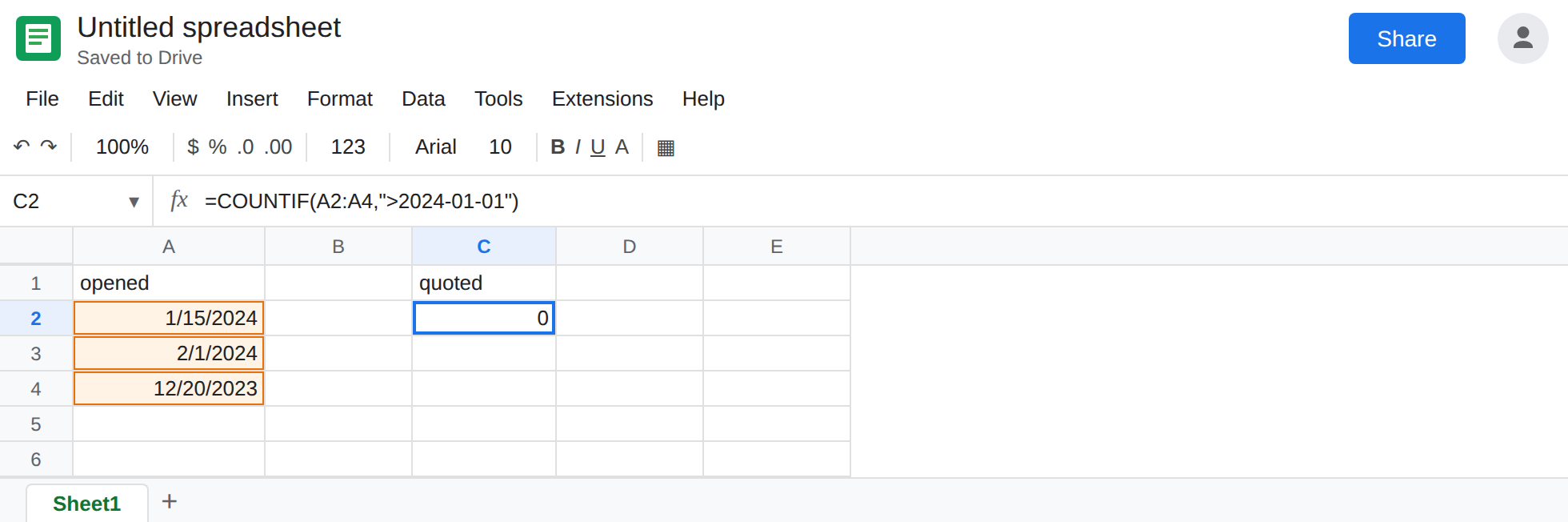
Quoted text criterion. In C1 type quoted. In C2 enter =COUNTIF(A2:A4,">2024-01-01"). The cell shows 0. The rows are on the sheet. The criterion never became a date comparison. Leave C2 as 0.

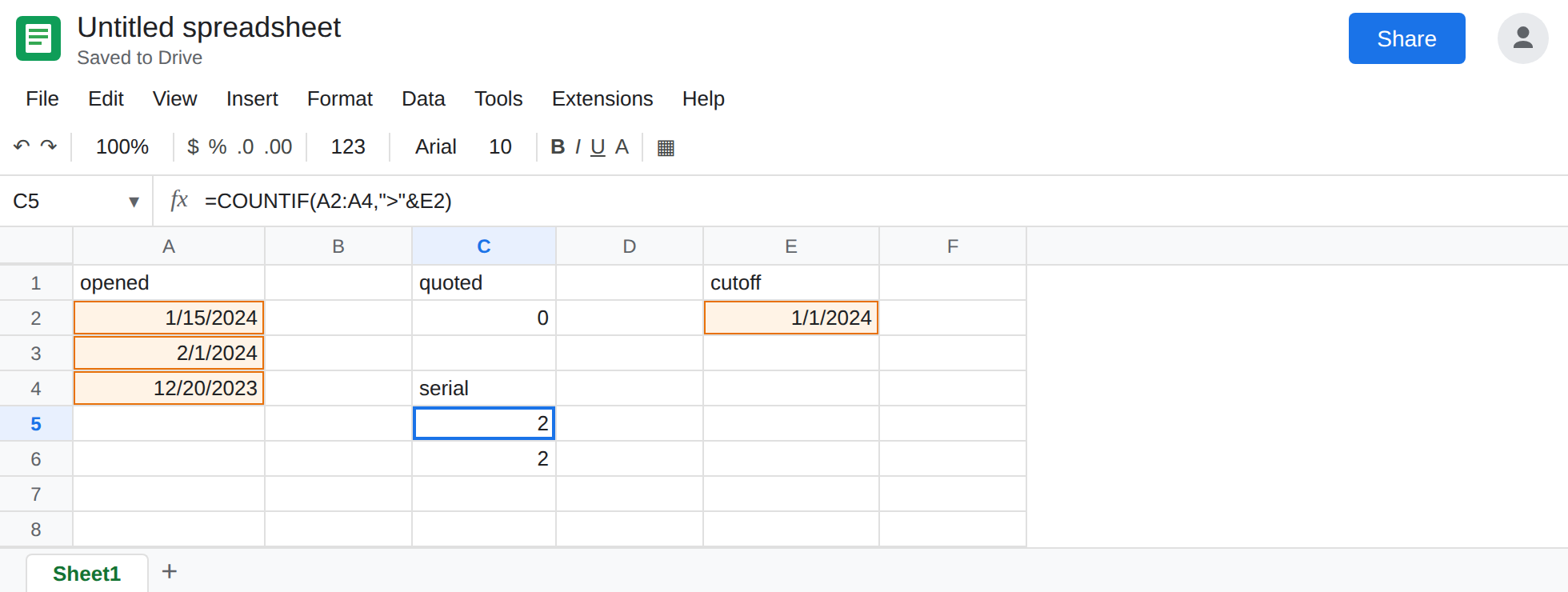
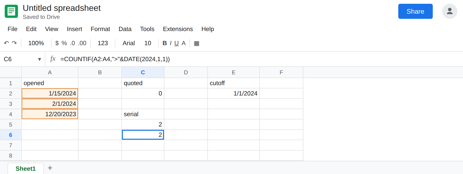
A date serial criterion. In E1 type cutoff. In E2 enter =DATE(2024,1,1). In C4 type serial. In C5 enter =COUNTIF(A2:A4,">"&E2). The cell shows 2 (15 Jan and 1 Feb). The operator is text. The date is a number. The & builds one criterion Sheets can apply to serials. In C6 enter =COUNTIF(A2:A4,">"&DATE(2024,1,1)). C6 is also 2. That pair is the control.

A text date still will not join this fix. In A6 type an apostrophe and then 2024-03-01, so the cell is left-aligned text. In C8 enter =COUNTIF(A6,">"&E2). C8 is 0. The criterion is now a real date comparison, and A6 is not a date. That miss is SUMIFS date text. Leave C8 as 0.

Leave C2 as 0. Leave C5 as 2.

What is actually wrong

• The quotes in ">2024-01-01" wrap the operator and the date together. COUNTIF does not pull 2024-01-01 out and run it through DATEVALUE for you. It compares a number (the serial in A2) with a text criterion. The count of matches is 0.
• ">"&E2 is a different value. E2 is a serial. Concatenating ">" with that serial produces a criterion whose right-hand side is numeric. C5 counts two rows. C6 is the same idea without a helper cell.
• >=, <, and <= have the same split. =COUNTIF(A2:A4,"="&DATE(2024,1,15)) can match A2. =COUNTIF(A2:A4,"=2024-01-15") stays on the text side with C2.
• Locale makes the quoted form worse, not better. ">1/2/2024" is month-day in one file and day-month in another, when it is parsed at all. DATE(2024,1,2) does not depend on that display order. See DATEVALUE day order for the parse, not for COUNTIF.
• A blank criterion cell makes ">"&E2 into ">" alone if E2 is empty. That is not “after 1 Jan.” Keep a real date in E2.

This is not #VALUE! from mismatched range sizes. See COUNTIFS range size. C2’s ranges are the same height. The result is a number.

This is not a wildcard. There is no * in the criterion. See COUNTIF literal * ?.

Fix

Leave C2 as the quoted 0.

Build the criterion from a date. Keep C5 or C6. For a window, =COUNTIFS(A2:A4,">="&DATE(2024,1,1),A2:A4,"<"&DATE(2024,2,1)) counts only January 2024 in this list (A2). COUNTIFS uses the same criterion rules. The range-size errors on that function are the other page.

If the count is still 0 with a serial criterion, the column is text. =ISTEXT(A6) is TRUE on the apostrophe cell. =ISNUMBER(A2) is TRUE on a real date. Convert with DATEVALUE only when the text is a date your locale accepts, then count the helper column. Do not expect C6 to include A6.

Do not wrap C2 in IFERROR. Zero is not an error. You would hide the only signal that the criterion is text.

If COUNTIF on dates is 0 and the formula bar shows the operator inside the same quotes as the date, move the operator out and join it to DATE or to a date cell. If the criterion is already a serial and the zeros remain, the cells are text and you are on the SUMIFS date page.