DGET returns #VALUE! for no match and #NUM! for more than one

DGET(database, field, criteria) returns one value from a table that has a header row. Zero matching records is #VALUE!. More than one matching record is #NUM!. The tooltip for the second case is More than one match found in DGET evaluation. A blank cell under a criteria header does not mean “ignore this column.” It means “this column may be anything,” which often matches every row and trips #NUM!.

This page is those two outcomes. It is not VLOOKUP no match (#N/A, and the first hit wins when several rows share a key). It is not FILTER no match. Keep the Google Sheets UI in English.

Recreate it on a blank sheet

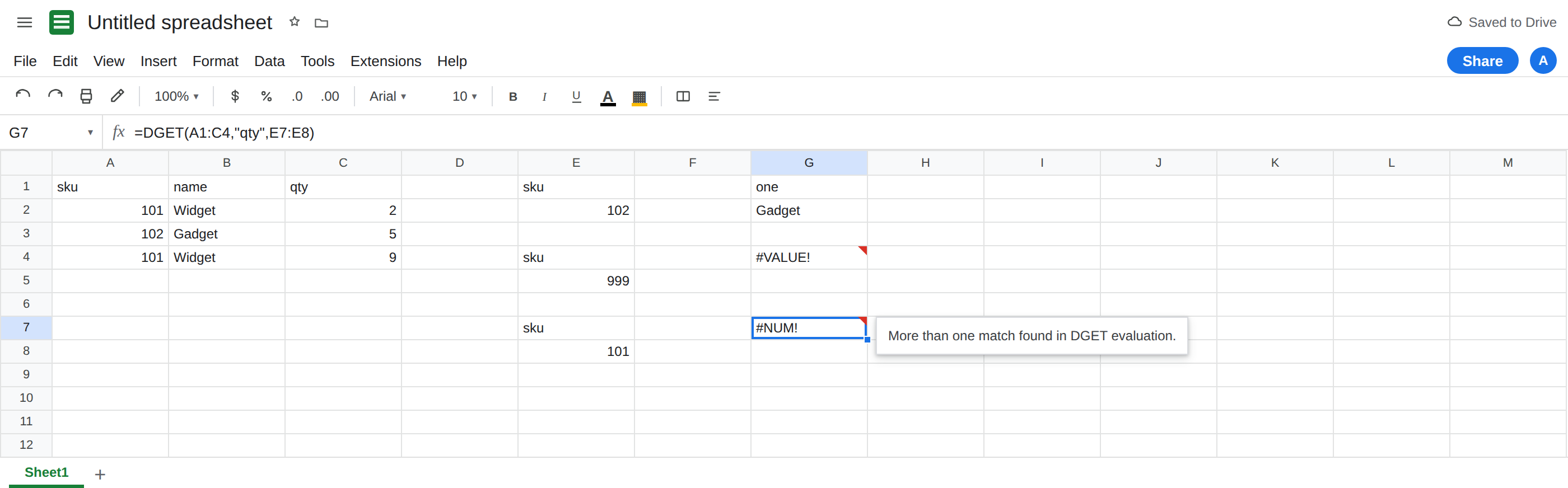
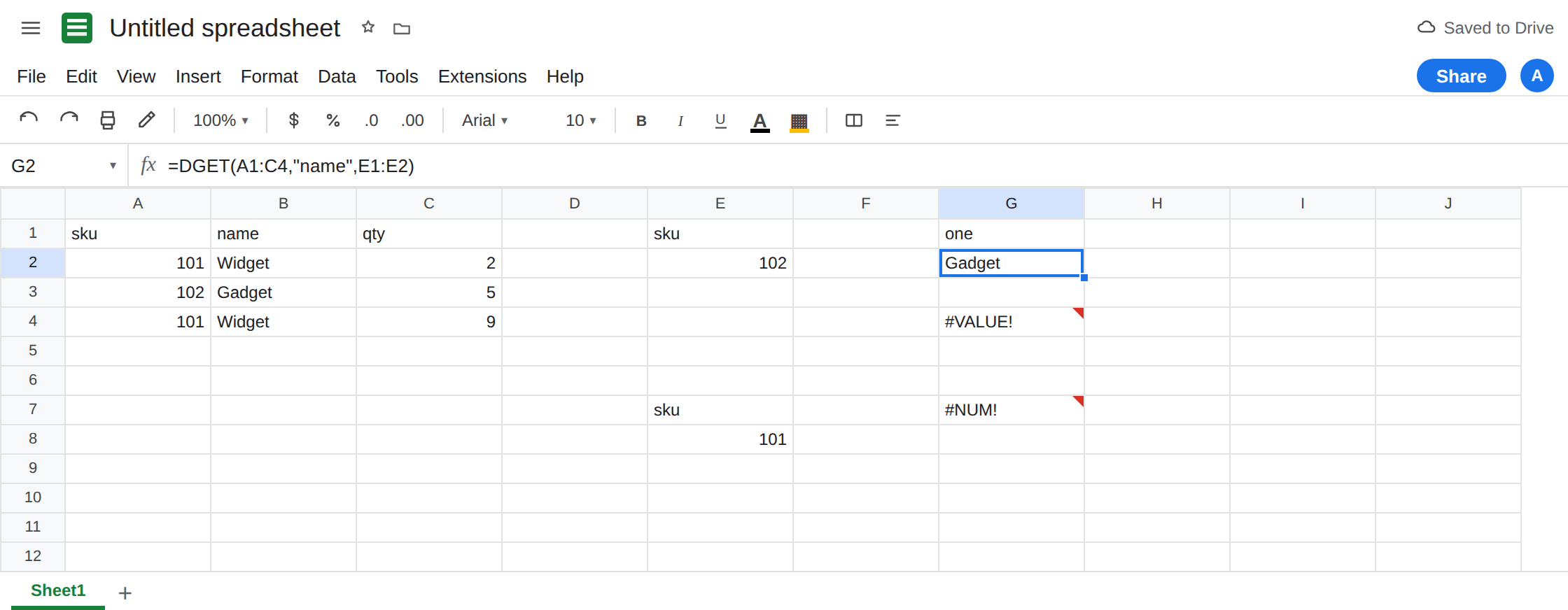
1. Open a blank spreadsheet. In A1 type sku, B1 name, C1 qty. A2 101, B2 Widget, C2 2. A3 102, B3 Gadget, C3 5. A4 101, B4 Widget, C4 9. Two rows share sku 101. The database is A1:C4, headers included.

One exact hit. In E1 type sku. In E2 type 102. In G1 type one. In G2 enter =DGET(A1:C4,"name",E1:E2). G2 is Gadget. The criteria range is a header plus one row. The field "name" is a header in the database. That cell is the control.

No such sku. In E4 type sku. In E5 type 999. In G4 enter =DGET(A1:C4,"name",E4:E5). The cell shows #VALUE!. Nothing in column A is 999. The tooltip is that no match was found in DGET. Leave G4 broken.

Two hits. In E7 type sku. In E8 type 101. In G7 enter =DGET(A1:C4,"qty",E7:E8). Rows 2 and 4 both match. The cell shows #NUM!. The tooltip is More than one match found in DGET evaluation. VLOOKUP of 101 would have returned the first qty, 2, with no error. DGET refuses to pick. Leave G7 broken.

A blank criterion. In E10 type sku. Leave E11 empty. In G10 enter =DGET(A1:C4,"name",E10:E11). An empty criterion under sku matches every data row. Three rows match. G10 is #NUM!, the multiple-match error, not a blank result and not “no filter.” Leave G10 broken.

Header mismatch. In E13 type SKU. In E14 type 102. In G13 enter =DGET(A1:C4,"name",E13:E14). If the criteria header does not match a database header, DGET does not filter on sku. You get #VALUE! or #NUM! depending on whether the unmatched criteria range selects nothing or everything. Do not assume the uppercase header is “close enough.” Leave G13 broken if it is not Gadget.

Field name. In G16 enter =DGET(A1:C4,"title",E1:E2). There is no header title. The cell errors (#VALUE!). Column index 2 is the name column: =DGET(A1:C4,2,E1:E2) is Gadget, the same as G2. A wrong label is not a wrong index.

Leave G4, G7, and G10 broken. Leave G2 as Gadget.

What is actually wrong

• DGET is the database function that will not aggregate. DSUM would add both qty values for sku 101. DGET returns #NUM! instead. The tooltip names DGET and “more than one match.” That is G7.
• No row is #VALUE!, not #N/A. Wrapping G4 in IFNA does nothing. See IFERROR vs IFNA. People coming from VLOOKUP reach for IFNA and the #VALUE! stays.
• Criteria are a range with headers. E1:E2 is header sku and value 102. Passing only E2 (102 with no header) is not a criteria range. Passing A2:C4 without its header row makes the first data row look like headers.
• A blank criteria cell is a wildcard for that column. G10 matches Widget, Gadget, and Widget again. If you meant “sku is empty,” the source does not have an empty sku. Delete the criteria row’s blank only after you put a real key in it, or stop calling DGET.
• Text criteria are not automatically exact. A key North can also match North East because database criteria treat the text as a prefix-style match. Force an exact comparison by putting = in front of the criterion. In a cell, type an apostrophe first so Sheets does not treat =102 as a formula: '=102. In an inline criteria array, =DGET(A1:C4,"name",{"sku";"=102"}) is exact. The apostrophe is only for the cell.

This is not QUERY returning #N/A for no rows. See QUERY no matching rows. Different function, different empty.

Fix

Leave G4, G7, and G10 broken.

One row, exact key. Keep G2: =DGET(A1:C4,"name",E1:E2) with E2 holding 102. For sku 101, do not ask DGET which qty is “the” qty. The table has two. Use =FILTER(C2:C4,A2:A4=101) to list 2 and 9, or =SUMIF(A2:A4,101,C2:C4) if you wanted 11. DGET is the wrong function when duplicates are real.

Fill or remove a blank criterion. G10 needs a sku in E11, or the formula should be deleted. Do not leave a criteria header sitting over an empty cell “for later.”

Exact text. Use '=Widget under a name header when a longer name might start with the same letters. Numeric 102 does not need that trick unless you are matching text that looks like 102.

Do not wrap G7 in IFERROR. You would hide a duplicate key and publish a blank qty. If the product requirement is “blank when it is not unique,” test the count first: =IF(COUNTIF(A2:A4,E8)<>1,"",DGET(A1:C4,"qty",E7:E8)). The COUNTIF tells you why.

If DGET is #NUM!, more than one row matched, including a blank criterion that matched all of them. If it is #VALUE!, nothing matched, or the field label is not a header. VLOOKUP will not teach DGET to return the first of two rows.