XLOOKUP returns the first duplicate and does not say there was another

XLOOKUP(key, lookup_range, return_range) stops at the first exact match when you omit search_mode. A second row with the same key does not raise #N/A and does not average the two results. The cell is simply the first row’s value. The sixth argument -1 walks from the bottom and returns the last duplicate instead. That -1 is not the fourth argument (if_not_found) and not the fifth (match_mode). Put it in the wrong slot and you are still on the first hit, or you have changed the match rule.

The last row is not “the latest date” unless the sheet happens to be in date order. That trap is XLOOKUP last row. Binary search modes are XLOOKUP binary. A key that is absent entirely is XLOOKUP #N/A. Keep the Google Sheets UI in English. Sheet Error is an independent formula-error library, not a Google product.

Recreate it on a blank sheet

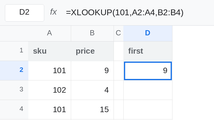
1. Open a blank spreadsheet. In A1 type sku, B1 price. A2 101, B2 9. A3 102, B3 4. A4 101, B4 15. Sku 101 is on two rows. The first price is 9. The last price is 15. Nothing says which price is current except the row order you are about to assume.

Default: first hit. In D1 type first. In D2 enter =XLOOKUP(101,A2:A4,B2:B4). D2 is 9. There is no triangle. 15 is on the sheet and did not get a turn, because row 2 already matched. Leave D2 as 9. That cell is the control, and it is the surprise: duplicates are legal.

-1 in the missing-value slot does not search upward. In D4 enter =XLOOKUP(101,A2:A4,B2:B4,-1). The fourth argument is what to return when the key is missing. The key is not missing. D4 is still 9. The -1 sits unused. In D5 enter =XLOOKUP(999,A2:A4,B2:B4,-1). D5 is -1. That is the fallback, not a price. Leave D4 as 9 so the misplaced -1 stays visible.

The sixth argument is the direction. In D7 enter =XLOOKUP(101,A2:A4,B2:B4,,,-1). Two commas skip if_not_found. Two more skip match_mode. -1 is search_mode. D7 is 15, the price on the last 101. Leave D7 as 15. It is the bottom row, not a sort by price. Swap B2 and B4 and D7 follows the new bottom row. It will not hunt for the larger number.

Both rows. In F1 type all. Leave F2:G3 empty. In F2 enter =FILTER(A2:B4,A2:A4=101). The spill is 101 / 9 and 101 / 15. XLOOKUP cannot return that spill. FILTER can. If you only needed to know the duplicate exists, =COUNTIF(A2:A4,101) is 2.

Leave D2 as 9. Leave D7 as 15. Leave D4 as 9.

What is actually wrong

• Omitted search_mode is first-to-last. The first exact 101 wins. A later 101 is not an error and not a tie-break. D2.
• Argument position matters more than the number -1. Fourth is the fallback for a miss (D4, D5). Fifth would be match_mode (2 means wildcards). Sixth is the direction. D7.
• Bottom-to-top returns the last duplicate in the range you passed. It does not sort that range. If the current price is the max, use MAXIFS or FILTER, not search_mode. The date version of this mistake is XLOOKUP last row.
• FILTER is the function that keeps every match. F2. XLOOKUP is the function that keeps one.
• An approximate match_mode of -1 or 1 in the fifth slot changes which nearby key is legal. That is XLOOKUP match_mode. It is not how you ask for the second duplicate.

This is not XLOOKUP binary. Search mode 2 or -2 requires sorted keys and can return a wrong row with no duplicate involved. D2’s keys are not sorted, and the default mode does not use binary search. The 9 is the true first 101.

Fix

Leave D2 as the first price and D7 as the last price.

Say which duplicate you want. Keep D2 when the contract is “the first 101 on the sheet.” Keep D7 when the contract is “the last 101 in this range.” Write first or last in the label. Do not put -1 in the fourth slot and call it last. D4 is still first.

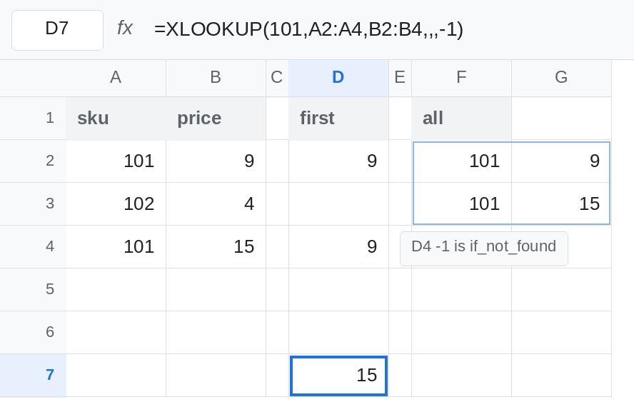
Every match, or the max price. F2 lists both rows. =MAXIFS(B2:B4,A2:A4,101) is 15 on this sheet because 15 happens to be the larger price, not because it is the last row. If you need the row that holds the max, MAXIFS still returns only the number. See MAXIFS returns the number.

A missing key should look missing. =XLOOKUP(999,A2:A4,B2:B4,"missing",,-1) is missing. The direction does not matter when nothing matches. "missing" in the fourth slot is a label. -1 in the fourth slot is a number that looks like a price. See XLOOKUP #N/A.

If the price is the upper row and you expected the lower row, you omitted search_mode. If you typed -1 and nothing changed, count the commas. The direction is the sixth argument. If both prices should have appeared, XLOOKUP is the wrong function. Use FILTER.