

MAXIFS returns the max number, not the rest of that row
Updated
MAXIFS(max_range, criteria_range, criterion) returns one number: the largest value in max_range among rows that pass the criteria. It does not return the name, the date, or any other column from that row. A cell that shows 40 is doing what MAXIFS does. The blank next to it is not a failed lookup. Nothing in MAXIFS accepts a “return column.”
OR criteria, which MAXIFS quietly turns into AND, are MAXIFS OR criteria. A #VALUE! from unequal range heights is MAXIFS / MINIFS size. A 0 when nothing matches is MINIFS / MAXIFS no match. Keep the Google Sheets UI in English. Sheet Error is an independent formula-error library, not a Google product.
Recreate it on a blank sheet
Section titled “Recreate it on a blank sheet”- Open a blank spreadsheet. In A1 type
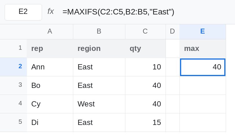
rep, B1region, C1qty. A2Ann, B2East, C210. A3Bo, B3East, C340. A4Cy, B4West, C440. A5Di, B5East, C515. East’s largest qty is40, and that row is Bo. West also has a40, on Cy. Two rows share the number40.
The max, which is only the number. In E1 type max. In E2 enter =MAXIFS(C2:C5,B2:B5,"East"). E2 is 40. It does not say Bo. There is no second argument for the rep column. Leave E2 as 40. That cell is the control: the aggregate is right, and it is still not a row.
XLOOKUP of that max hits the wrong tie. In E4 enter =XLOOKUP(E2,C2:C5,A2:A5). E4 is Bo on this sheet only because Bo’s 40 sits above Cy’s 40. The lookup is “first qty equal to 40,” not “the East row whose qty is the East max.” If you sort Cy above Bo, E4 becomes Cy while E2 stays 40. The max did not move. The name lookup walked the qty column with no region test. Leave E4 as that name and do not trust it as the East rep.
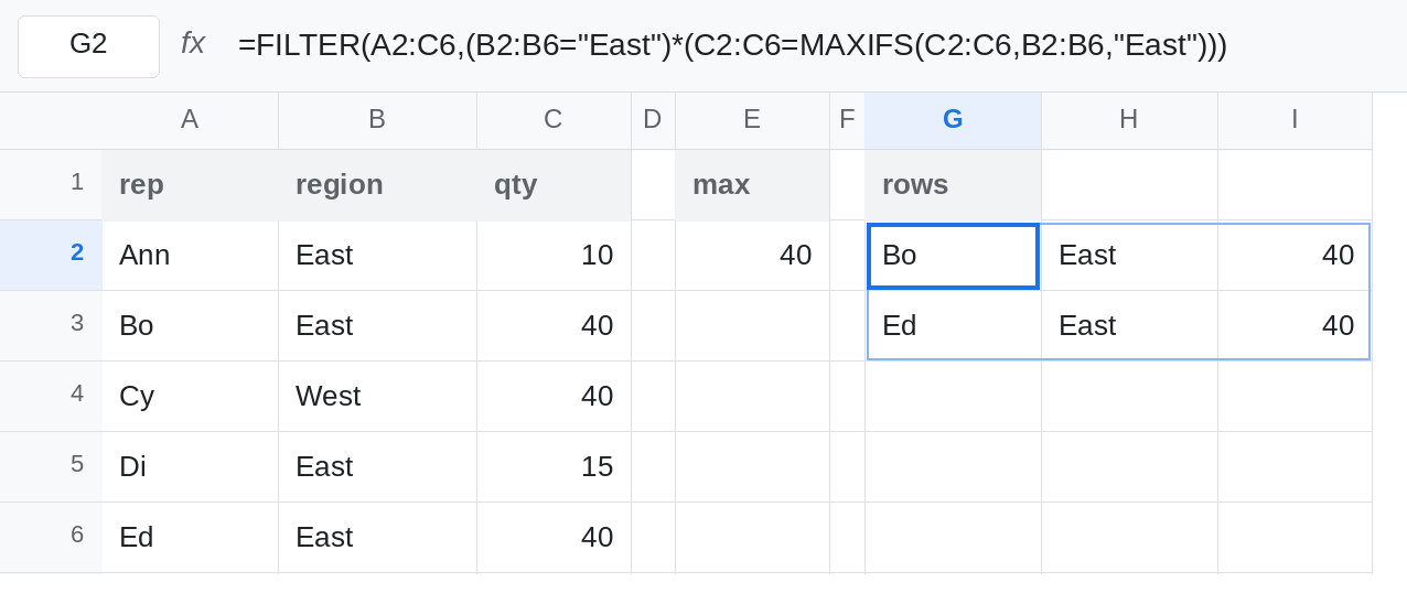
FILTER keeps every tied row that passes. In G1 type rows. Leave G2:I4 empty. In G2 enter =FILTER(A2:C5,(B2:B5="East")*(C2:C5=E2)). The spill is one row: Bo, East, 40. Cy is 40 and is not East, so Cy is out. Add another East 40: in A6 type Ed, B6 East, C6 40. G2 spills Bo and Ed. MAXIFS in E2 is still 40. The aggregate cannot tell you there are two reps. Leave the second East 40 in place if you want both rows visible.
SORTN returns one row unless ties are requested. In G6 enter =SORTN(FILTER(A2:C6,B2:B6="East"),1,0,3,FALSE). The third argument of SORTN is the tie mode. 0 returns exactly one row: the top East qty. The 3 is the qty column inside the filtered block, and FALSE is descending. You get one of Bo or Ed, not both. Tie mode 2 returns every row tied for that top qty. That flood is SORTN ties mode and SORTN tie flood.
Leave E2 as 40. Leave E4 as a name that did not check region.
What is actually wrong
Section titled “What is actually wrong”MAXIFSis an aggregate. The result is a scalar frommax_range. Rep, region, and date are not in the return value, even when they sat on the winning row.- Looking up the scalar in the qty column drops the criteria. E4 can return a West rep who happens to share the number. Ties make that lookup unstable as soon as the sheet is sorted.
FILTERwith the criteria andqty=MAXIFS(...)returns every matching row. Two East reps at40are two rows. That is the list. It is#N/Aonly when no row matches. See FILTER no match.SORTNof that filtered block is how you ask for the top row instead of the top number. Tie mode0hides the tie. Tie mode2shows it. Pick the mode in the formula, not after the chart looks short.- A second criteria pair inside
MAXIFSis AND, not a way to return another column. See MAXIFS OR criteria.
This is not MAXIFS returning 0 because East is missing. E2 is 40. The missing piece is the row.
Leave E2 as the scalar. Leave E4 as the unsafe name lookup.
The East row or rows. Keep G2: =FILTER(A2:C6,(B2:B6="East")*(C2:C6=MAXIFS(C2:C6,B2:B6,"East"))). You do not need E2 as a helper. With Bo and Ed both at 40, the spill is two rows. Index the rep only when you have decided that one row is enough: =INDEX(G2,1,1) after the spill, or use SORTN below.
One top row, ties called out. =SORTN(FILTER(A2:C6,B2:B6="East"),1,2,3,FALSE) uses tie mode 2, so every East rep tied at the top qty is returned, and reps below that qty are not. Mode 0 is the single-row version. See SORTN n / ties.
Put the region test in the lookup if you refuse FILTER. =XLOOKUP(1,(B2:B6="East")*(C2:C6=E2),A2:A6) returns the first East rep at that qty. A later tie is dropped. Say so in the header. Default XLOOKUP on the qty column alone is E4, which is the bug.
Do not wrap E2 in INDEX and hope a name appears. MAXIFS did not spill a row. If the number is right and the name is wrong, the name came from a lookup that forgot the criteria or forgot the tie.