A pivot calculated field multiplies the totals, and a cell reference is not a field

A pivot calculated field is a formula on source field names, computed from the values the pivot has already aggregated for that group. ='qty'*'price' for East is (2+3)*(10+4), which is 70. The line totals are 2*10 and 3*4, and their sum is 32. The pivot did not do the multiplication per source row and then add. It multiplied the group totals. A formula written with cell addresses, =B2*C2, is not those field names. Sheets has nothing in the pivot source named B2. The field fails, shows a blank, or returns an error, and the relative reference never walks down the source the way a sheet formula would.

A pivot that keeps old totals is pivot not refreshing. GETPIVOTDATA on a grouped date is GETPIVOTDATA month. Keep the Google Sheets UI in English. Sheet Error is an independent formula-error library, not a Google product.

Recreate it on a blank sheet

1. Open a blank spreadsheet. In A1 type region, B1 qty, C1 price. A2 East, B2 2, C2 10. A3 East, B3 3, C3 4. A4 West, B4 1, C4 10. Line totals are 20, 12, and 10. East’s line totals add to 32. East’s summed qty is 5 and East’s summed price is 14. Five times fourteen is 70.

The pivot. Select A1:C4. Insert → Pivot table on the same sheet, starting at E1. Rows: region. Values: qty summarized by SUM, and price summarized by SUM. East shows qty 5 and price 14. West shows qty 1 and price 10. Those sums are what a calculated field will see.

The calculated field people expect to be 32. In the pivot editor, under Values, Add → Calculated field. In the formula box enter ='qty'*'price'. Field names are the headers, in single quotes. Name it ext if the editor asks. East’s calculated value is 70, not 32. West’s is 1*10, which is 10, and it matches the only West line, so West hides the bug. Leave the East 70 on the pivot.

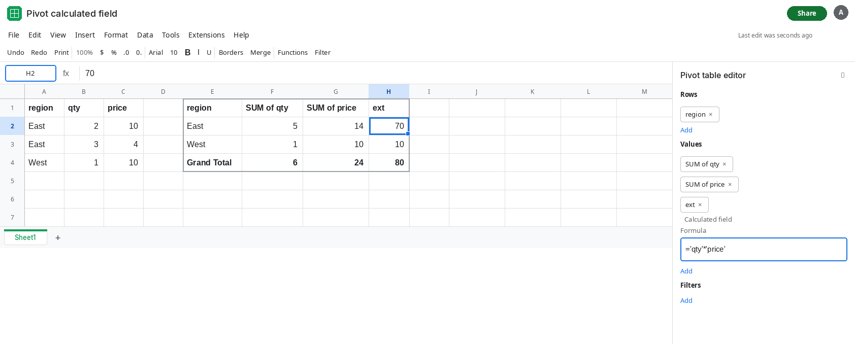
A cell reference is not a field. Edit the calculated field to =B2*C2. Those are cells on the grid, not headers in the source. The pivot does not fill that formula down A2:C4. You get an error, a blank value, or a result that ignores the source rows. Put the formula back to ='qty'*'price' so the 70 is what you are looking at. If your editor accepted B2*C2 and shows a single number, it is not the sum of line totals. Compare it to 32.

SUM of qty and SUM of price are not the bug. The 5 and the 14 are correct sums. The surprise is only the product of those sums. Adding the two fields, ='qty'+'price', would show 19 for East (5+14), which is a fair sum of sums. Multiplication and division are where the order of operations changes the meaning.

Leave the calculated field showing 70 for East.

What is actually wrong

• The calculated field runs after the grouping. Each field name in the formula stands for that field’s aggregate in the group, not for each source row. Product of sums is not sum of products. Excel calculated fields have the same order. A sheet formula copied from column D does not keep its row-by-row behavior inside the pivot.
• Quotes around the header are how Sheets names a field. qty without quotes can be read as a name that is not a field. B2 is a cell. The source has no column headed B2.
• One-row groups hide the bug. West has a single line, so sum of products and product of sums match. Always check a group with two different prices.
• The field cannot see another pivot cell, a GETPIVOTDATA result, or a sheet range off to the side as a normal relative fill. People who need a price list lookup do that on the source, in a helper column, before the pivot. A lookup typed into the calculated field is a different, brittle setup. This page is the aggregate-then-multiply limit.
• Refreshing the pivot recalculates 70. It will not start doing row-level products. See pivot not refreshing only when the 5 and the 14 themselves are stale.

This is not SUMPRODUCT on the sheet. =SUMPRODUCT((A2:A4="East")*(B2:B4)*(C2:C4)) is 32, because it multiplies per row. The pivot formula is not that.

Fix

Leave the calculated field at 70 so the product-of-sums stays visible.

Add the line total on the source, then sum it. In D1 type line. In D2 enter =B2*C2 and fill D2:D4. D2 is 20, D3 is 12, D4 is 10. In the pivot editor, change the data range to A1:D4 if it did not expand. Remove the calculated field or leave it as the broken example. Add Values: line, summarized by SUM. East’s line sum is 32. West’s is 10.

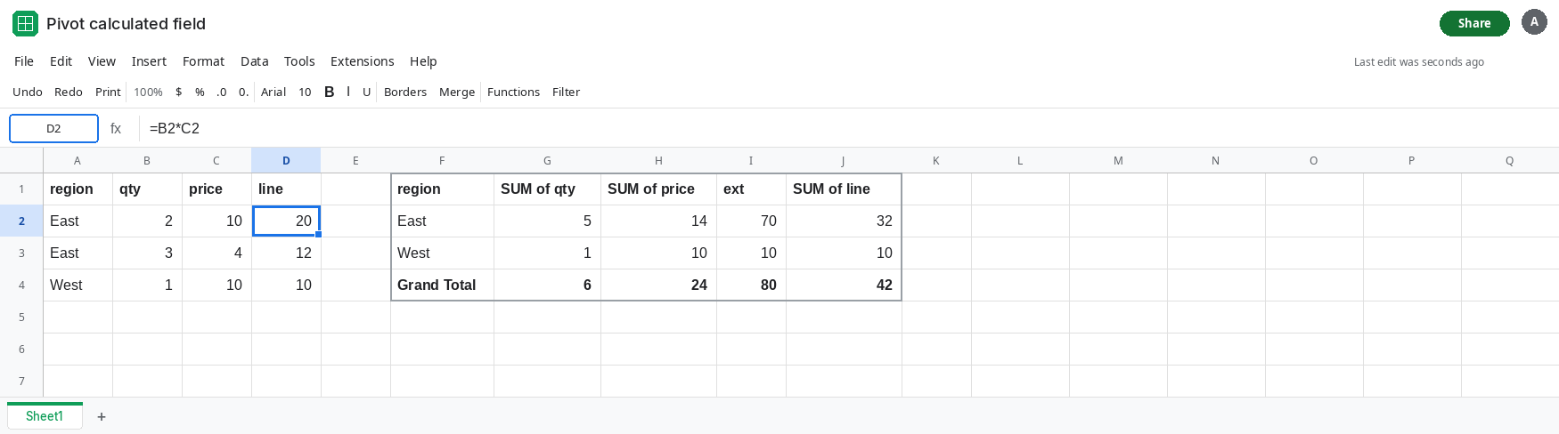
Keep a calculated field for math that is safe on aggregates. A ratio of two sums, such as total qty over a count of rows, is a question about the aggregates. A margin that must be quantity times price per order is a helper column. If you divide summed revenue by summed units you get a weighted average price, which is sometimes what you wanted. Write the header so it does not say “line total.”

If East shows 70 for ='qty'*'price' and the source lines add to 32, the field multiplied the totals. If the formula box contains B2 or C2, those are not source fields. If the helper column sums to 32 and the pivot still shows the old range, the data range does not include column D yet.