Fix FILTER #VALUE! or #N/A from mismatched range sizes in Google Sheets

FILTER needs every condition to be the same height as the data range. A condition that is one row taller or shorter is an error. In the English Google Sheets UI that cell is usually #N/A, tooltip FILTER has mismatched range sizes. Some callers also see #VALUE!. Either way, this is a size failure. It is not “zero matching rows.”

This page is mismatched heights. It is not FILTER no match (sku 999 with equal heights; tooltip No matches are found in FILTER evaluation). It is not COUNTIFS range size (COUNTIFS / SUMIFS size errors are #VALUE! with Array arguments to COUNTIFS are of different size).

Recreate it on a blank sheet

1. Open a blank spreadsheet. In A1 type lane, B1 crate. A2 L1. B2 N12. A3 L2. B3 N18. A4 L1. B4 N21. Three data rows.

Height mismatch. In D1 type mismatch. In D2 enter =FILTER(A2:B4,A2:A5="L1"). A2:B4 is three rows. The condition A2:A5 is four. The cell shows #N/A (sometimes #VALUE!). The tooltip is FILTER has mismatched range sizes. Expected row count: 3. column count: 1. Actual row count: 4, column count: 1. Lane L1 is on the sheet. Leave D2 broken.

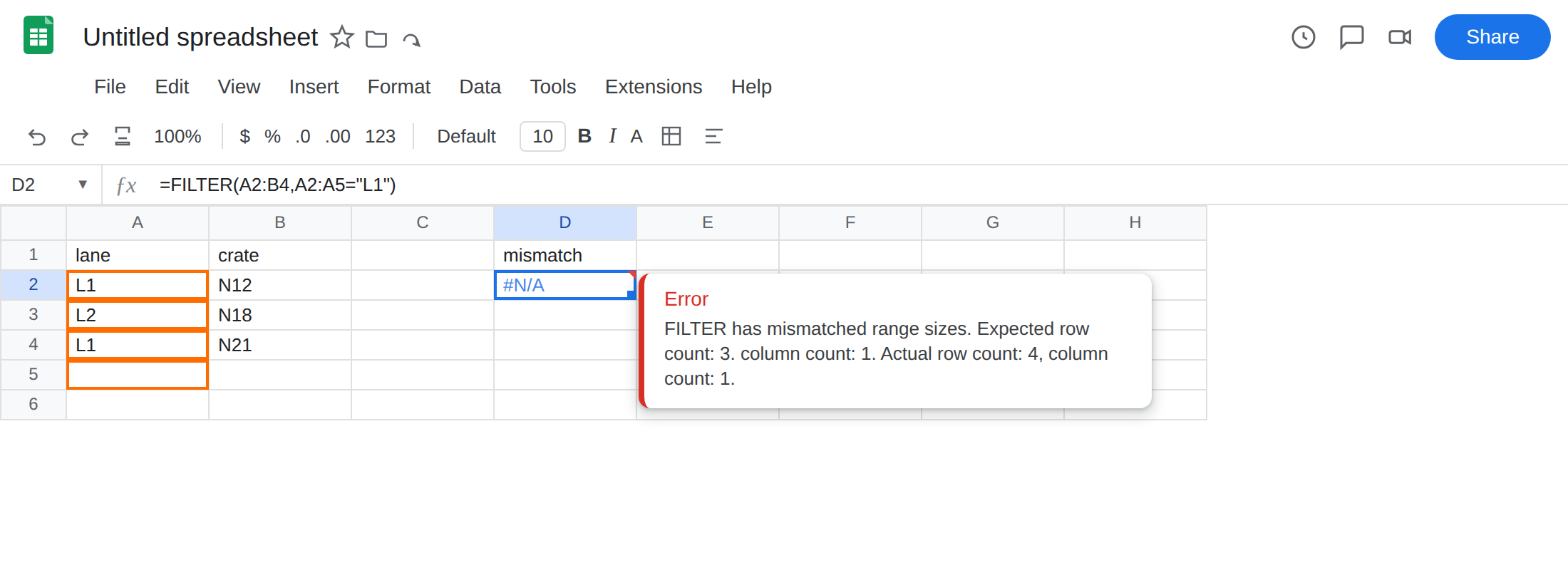
Open column vs a bounded range. In D5 type open. In D6 enter =FILTER(A2:B4,A2:A="L1"). A2:A runs to the bottom of the sheet. A2:B4 is three rows. Same size error. Leave D6 broken.

Equal heights, a real miss — not this page. In F1 type no_match. In F2 enter =FILTER(A2:B4,A2:A4="L9"). Heights match (three and three). L9 is not in the lane column. The cell shows #N/A. The tooltip is No matches are found in FILTER evaluation. Leave F2 as the contrast. That tooltip is FILTER no match. Do not wrap D2 the way you wrap F2.

Confirm the size error. Change "L1" to "L9" on D2. The error stays. On F2, changing "L9" to "L1" spills two rows. That toggle is the no-match page.

Two conditions, second one tall. In H2 enter =FILTER(A2:B4,A2:A4="L1",B2:B5="N12"). Same size tooltip. Leave H2 broken.

What is actually wrong

• FILTER(range, condition) walks the condition in lockstep with the rows of range. Three data rows next to four condition rows is a size error. Sheets refuses the shapes before it filters. Lane L1 never gets a chance to match.
• An open-ended column (A2:A or A:A) is not the same height as A2:B4. Mixing them is the same error.
• Two conditions must each match the data height. A legal first condition does not save a tall second condition.
• The error value is usually #N/A, the same token as an empty FILTER. The tooltip is the split. Read it. Expected row count / Actual row count is this page. No matches are found is the other page.
• #VALUE! here, if you see it, is still a shape problem. See wrong type only if the formula is arithmetic.

This is not zero matching rows. F2 is that recreate. See FILTER no match. IFNA is correct for F2. IFNA on D2 prints none and leaves the heights wrong.

This is not COUNTIFS / SUMIFS with ranges of different length. Those functions return #VALUE! (or a quiet 0 if the windows are the same size but shifted). See COUNTIFS range size. Do not copy a COUNTIFS fix onto FILTER and expect the error value to match.

This is not a VLOOKUP miss. See what #N/A means. FILTER is not searching with a column index.

Fix

Leave D2, D6, and H2 broken so the size error stays on the sheet. Leave F2 as the no-match contrast.

Make every range the same height. Same start row. Same end row. In E1 type filter_ok. In E2 enter =FILTER(A2:B4,A2:A4="L1"). The formula spills L1 / N12 and L1 / N21.

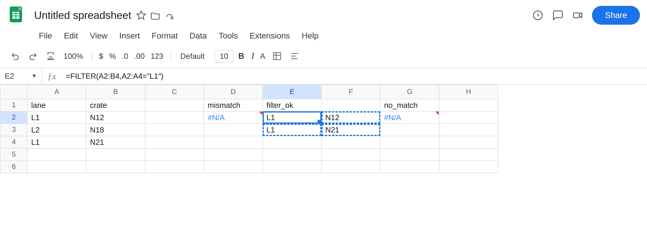
Open columns: open all of them, or none. If the table should grow, use A2:B with A2:A, not A2:B4 next to A2:A. In E6 enter =FILTER(A2:B,A2:A="L1"). That spills the two L1 rows and stays valid as you add A5. Do not mix a trailing A with a closed A2:B4.

Two conditions: same window. In I2 enter =FILTER(A2:B4,A2:A4="L1",B2:B4="N12"). One row spills. H2 stays broken.

Do not wrap D2 in IFNA or IFERROR. That prints a blank and never equalizes the heights. See IFERROR vs IFNA. Do not switch this formula to COUNTIFS to “get a #VALUE! you recognize.” Do not change File → Settings locale.

If the tooltip is FILTER has mismatched range sizes, count the rows in the formula bar. Make them the same. Then, if the cell is still #N/A, read the tooltip again — you may have moved onto FILTER no match.

Why FILTER mismatch is #N/A (and COUNTIFS is #VALUE!)

FILTER is an array that either spills rows or does not. Sheets used #N/A for “this FILTER produced nothing I can spill,” and reused that token for “I will not even try, the shapes disagree.” Same error value, two tooltips. That is why a wrapper that is correct for an empty filter is dangerous on a size bug.

COUNTIFS and SUMIFS are scalar counters. A length mismatch is #VALUE! (Array arguments … different size). That is COUNTIFS range size. If you remember “size = #VALUE!” from those functions, FILTER will surprise you. Trust the tooltip, not the token. Equal heights first. Empty results second.