Fix INDEX surprises in Google Sheets when the row or column is 0

INDEX(reference, [row], [column]) counts from the top-left of the range you passed, starting at 1. Row 0 is legal. It does not mean “first row,” and it is not an out-of-range error. It means all rows of the chosen column. Column 0 means all columns of the chosen row. The result is an array. If a neighbor is occupied, that array cannot spill and the cell is #REF!. An index past the last row is a different #REF!: the tooltip says the value is outside 0 through the size of the range.

This page is index 0 and the spill it creates. It is not INDEX past range as the primer for index 4 on a three-row block. It is not two-way lookup. Keep the Google Sheets UI in English.

Recreate it on a blank sheet

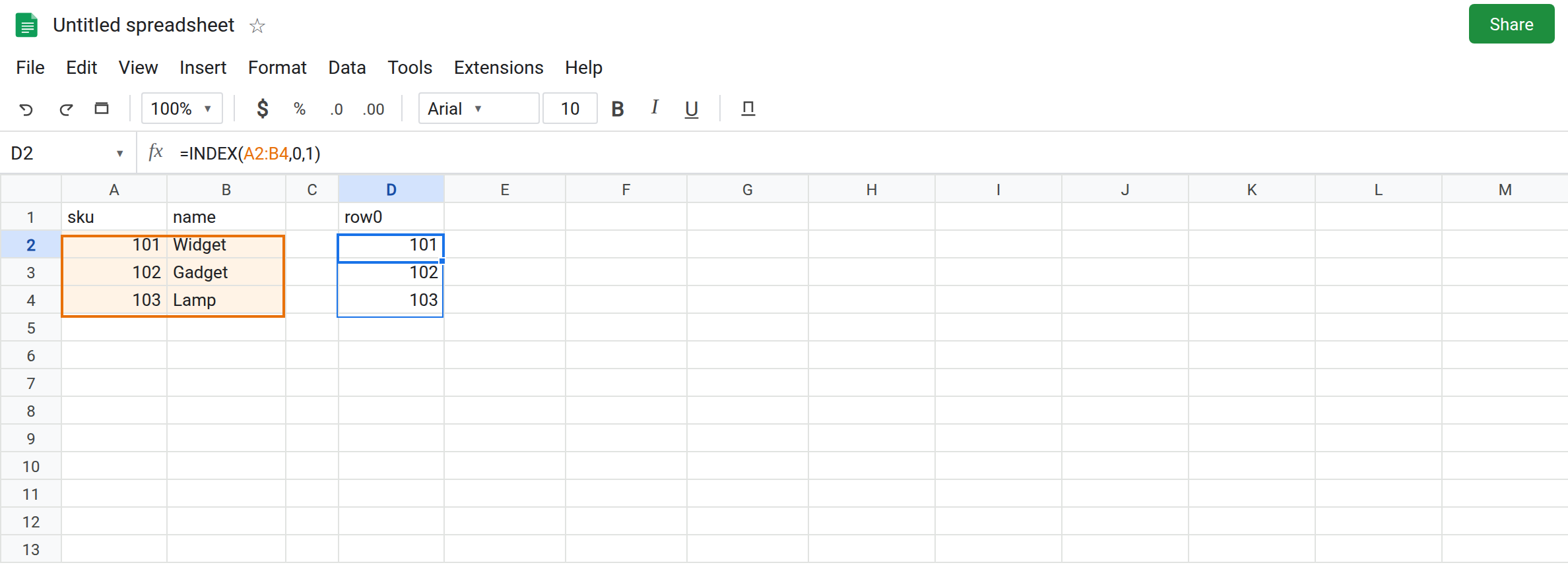
1. Open a blank spreadsheet. In A1 type sku, B1 name. A2 101, B2 Widget. A3 102, B3 Gadget. A4 103, B4 Lamp. The body A2:B4 is three rows and two columns.

Row 0 spills the column. In D1 type row0. Leave D2:D4 empty. In D2 enter =INDEX(A2:B4,0,1). Row argument 0, column 1. The formula spills 101, 102, 103 down from D2. You asked for “row zero” and received every sku. No error triangle when the path is empty. That spill is the surprise, and it is the control for what 0 means.

The same 0, blocked. In F1 type block. In F3 type keep. Leave F2 empty. In F2 enter =INDEX(A2:B4,0,1). A full column needs F2:F4. F3 is occupied. F2 shows #REF!. The tooltip is Array result was not expanded because it would overwrite data in F3. The index 0 was legal. The landing cells were not. Leave F2 broken.

Column 0. In H1 type col0. Leave H2:I2 empty. In H2 enter =INDEX(A2:B4,1,0). Column argument 0, row 1. The spill is one row: 101 and Widget. All columns of the first body row. If I2 had a value, H2 would be the same overwrite #REF! as F2, sideways.

Zero from a MATCH that you decremented. In A6 type 101. In D6 enter =MATCH(A6,A2:A4,0). The cell shows 1 (first body row). In D7 enter =INDEX(B2:B4,D6-1). 1-1 is 0. INDEX of column B2:B4 with row 0 spills Widget, Gadget, and Lamp if the cells below D7 are empty. You wanted the name on the previous row. There is no previous row. You got the entire name column. Leave D7 as that spill.

Past the range, for contrast. In D10 enter =INDEX(A2:B4,4,1). The cell shows #REF!. The tooltip says parameter 2 value is 4 and valid values are between 0 and 3 inclusive. 0 is inside that sentence. 4 is not. That tooltip is INDEX past range. Leave D10 broken so the two #REF! tooltips can be compared with F2. F2 names a cell. D10 names a parameter.

Leave F2 and D10 broken. Leave D2 as 101, 102, 103.

What is actually wrong

• 0 is documented as “the whole axis,” same as omitting that argument in the cases Sheets allows. It is inside the valid range. Programming habit (first item is index 0) does not apply. The first sku is index 1.
• A whole column is three cells here. It spills. Occupied F3 turns a legal 0 into overwrite #REF!. Clearing the index will not fix F2. Clearing F3 will.
• MATCH is 1-based. Subtracting 1 to mean “the row above” produces 0 on the first hit. D7 then dumps the column. Test the match before you subtract. If it is 1, there is no previous row.
• Both arguments 0 (INDEX(A2:B4,0,0)) returns the whole block. That is a 3×2 spill, not a single sku.
• A negative index is outside the tooltip’s range. #REF!, and the valid values still start at 0. Do not “fix” a negative by assuming Sheets will count from the bottom. This is not CHOOSEROWS. See CHOOSEROWS negative.

This is not VLOOKUP column index 3 on a two-column range. See VLOOKUP bad index. The function name in the formula bar is INDEX.

This is not a deleted reference. See after you delete. F2 still says INDEX.

Fix

Leave F2 and D10 broken. Leave D2 as the whole-column spill so 0 stays visible.

Ask for one cell with a 1-based index. In J1 type one. In J2 enter =INDEX(A2:B4,1,1). The cell shows 101. Relative row 1, relative column 1. For the name on the matched row, =INDEX(B2:B4,D6) with D6 equal to 1 shows Widget. Do not subtract 1.

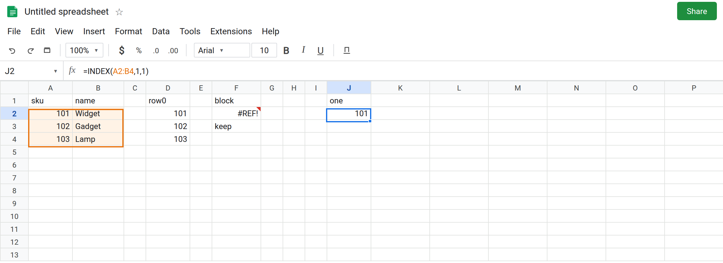
If you wanted the whole column, clear the path. Delete F3 or move the formula. F2’s formula can match D2 once F3 is empty. Do not change 0 to 1 if the column was the goal.

Previous row. =IF(D6<=1,"",INDEX(B2:B4,D6-1)). The IF stops the 0. It does not run INDEX with a zero row.

Do not wrap F2 in IFERROR. The column is real and the neighbor is in the way. See IFERROR vs IFNA.

If INDEX spills a column you did not expect, the row argument is 0 or omitted. If the tooltip says valid values are between 0 and n, the index is past n. If the tooltip names a cell that would be overwritten, 0 already meant “whole axis” and the spill is blocked.