IMAGE mode, height, and width: a blank-looking cell or a stretched picture

IMAGE(url, mode, height, width) puts a picture in a cell. mode is 1, 2, 3, or 4. Mode 1 fits inside the cell and keeps the aspect ratio. Mode 2 stretches to the cell and can distort the picture. Mode 3 uses the original pixel size, which can look cropped or like it overflowed. Mode 4 needs a height and a width in pixels. Mode 5, or mode 4 with the sizes omitted, errors. A short row plus mode 1 can look blank even when the URL is fine.

A URL that does not load is IMAGE failed to load. This page assumes a URL that already draws, then changes mode and size. Keep the Google Sheets UI in English. The sample URL below is the public PNG from Google’s own IMAGE help example. Use an image you are allowed to embed. Do not hotlink a random photo.

Recreate it on a blank sheet

1. Open a blank spreadsheet. In A1 type url. In A2 type https://www.google.com/images/srpr/logo3w.png. If Allow access appears on the first IMAGE, click it once.

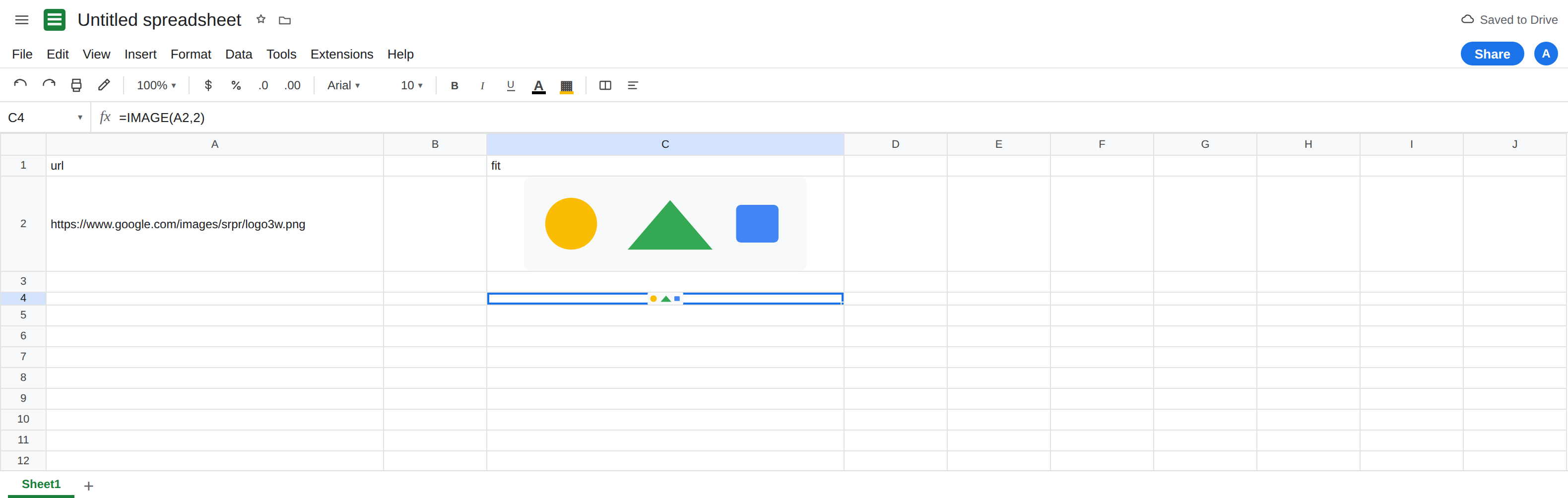
Mode 1, the fit. In C1 type fit. Make row 2 tall enough to see a logo (drag the row border). In C2 enter =IMAGE(A2,1). C2 shows the logo inside the cell, aspect ratio kept. That cell is the control. If C2 is #N/A and the tooltip says the URL could not be fetched, stop and use IMAGE failed to load. Mode will not repair a dead address.

Mode 2 stretches. In C4 enter =IMAGE(A2,2). Resize row 4 to be very short and column C to be very wide, or the reverse. The logo’s proportions change to fill the cell. There is no error triangle. The distortion is the mode. Leave C4 as the stretched picture.

Mode 4 without sizes. In E1 type custom. In E2 enter =IMAGE(A2,4). The cell errors (#N/A / #VALUE!). Mode 4 requires height and width. The tooltip says those parameters are missing or invalid. Leave E2 broken.

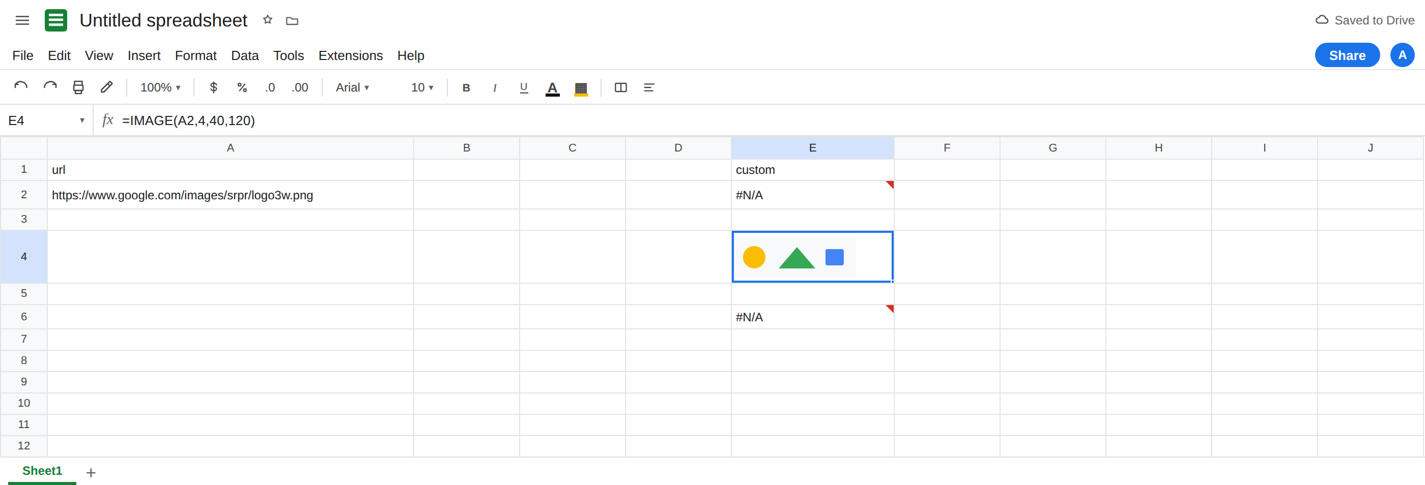
Mode 4 with sizes. In E4 enter =IMAGE(A2,4,40,120). E4 shows the logo at 40 pixels tall and 120 pixels wide. That is the custom-size control. The cell’s row height still has to be large enough to see it. A 40-pixel image in a 10-pixel row looks clipped or blank. Raise the row. Do not change the URL.

Mode 5. In E6 enter =IMAGE(A2,5). The cell errors. The tooltip is that parameter 2 must be between 1 and 4. Leave E6 broken. Height and width do not make 5 legal: =IMAGE(A2,5,40,120) still errors.

Mode 1 ignores the pixel arguments. In E8 enter =IMAGE(A2,1,40,120). This draws mode 1 (fit to the cell). The 40 and 120 are not applied. People add sizes and keep mode 1, then decide IMAGE is broken because the picture did not become 120 pixels wide. It is mode 1. Compare it with E4.

A short row that looks empty. Set row 10 to the default height. In C10 enter =IMAGE(A2,1). The logo is fitted into a short cell and can look like a speck or a blank. The formula is the same family as C2. Select C10 and look at the formula bar before you replace the URL.

Leave E2 and E6 broken. Leave C2 and E4 showing the logo.

What is actually wrong

• Mode 1 preserves aspect ratio and stays inside the cell. A short row shrinks the picture. The fix is row height, or mode 4 with a pixel height you can see. It is not a new URL.
• Mode 2 fills the cell and drops the aspect ratio. Wide cell, short row, stretched logo. That is what mode 2 is for. Use it only when distortion is acceptable.
• Mode 3 keeps the file’s pixel size. A large PNG overflows the cell and can cover neighbors. That overlap is not a #REF! spill from SORT. It is the image drawing outside. Mode 1 or 4 puts it back in a box.
• Mode 4 is the only mode that reads height and width, and it needs both, in pixels, greater than 0. Omitting them is E2. A height of 0 is an error. Passing sizes with mode 1 does not switch you to mode 4.
• Mode 5 is outside 1–4. The URL is not consulted once the mode is illegal, or the URL loads and the mode still fails. Either way E6 is the mode, not IMAGE failed to load.

This is not SPARKLINE. See SPARKLINE chart type. A chart has no mode 4.

Fix

Leave E2 and E6 broken.

Fit, or set pixels on purpose. Keep C2: =IMAGE(A2,1) and make the row tall enough. For a fixed size, keep E4: =IMAGE(A2,4,40,120). Change 40 and 120 together if you need a different box. To keep the aspect ratio at a chosen height, use mode 4 with a width that matches the picture, or stay on mode 1 and resize the cell.

Stretch only when you mean it. C4 is mode 2. Switch it to 1 if the logo should not be distorted. Do not “correct” the URL.

Do not wrap E2 in IFERROR. A missing size and a dead URL would both become blank, and a blank image cell looks like mode 1 in a short row. See IFERROR vs IFNA. Check the formula bar.

If the picture is tiny or stretched and the URL loads in another cell, read mode. 1 fits, 2 stretches, 4 needs both pixel sizes. If the tooltip says the image could not be fetched, you are on the URL page. Mode 5 will not start loading a better file.